Activation Functions
The activation function define the output of a node/neuron given its input signals. It do not participate in the backpropagation process, but it can affect the convergence of the model.
Binary Step Function
Binary step funciton is either on or off and it can not handle multiple classification abd the vertical slopes don’t work well with calculus. It is not used in practice.
Non-linear Activation Function
Non-linear activation functions are used to introduce non-linearity into the model, which allows it to learn more complex patterns in the data. And grace to it, we can stack multiple layers of neurons to create deep neural networks otherwise the stack of linear layers would still be a linear model.
Sigmoid Function: $$\sigma(x) = \frac{1}{1 + e^{-x}}$$ (0, 1) range, used for binary classification problems. It can cause vanishing gradient problem when the input is very large or very small.
Derivative: $$\sigma’(x) = \sigma(x)(1 - \sigma(x))$$
Tanh Function: $$\tanh(x) = \frac{e^x - e^{-x}}{e^x + e^{-x}}$$ (-1, 1) range, zero-centered, used for hidden layers. It can also cause vanishing gradient problem when the input is very large or very small.
Derivative: $$\tanh’(x) = 1 - \tanh^2(x)$$
ReLU Function: $$f(x) = \max(0, x)$$ Derivative: $$f’(x) = \begin{cases} 0 & \text{if }x < 0 \ 1 & \text{if } x > 0 \end{cases}$$ Very popular for hidden layers, it can help with the vanishing gradient problem, easy to compute, but it can cause the “dying ReLU” problem where neurons can get stuck in the inactive state and never recover.
Leaky ReLU Function: $$f(x) = \begin{cases} \alpha x & \text{if }x < 0 \ x & \text{if } x > 0 \end{cases}$$ Derivative: $$f’(x) = \begin{cases} \alpha & \text{if }x < 0 \ 1 & \text{if } x > 0 \end{cases}$$ It introduces a small slope for negative inputs, which can help prevent the “dying ReLU” problem and allow the model to learn from negative inputs.
Parametric ReLU (PReLU) Function: $$f(x) = \begin{cases} \alpha x & \text{if }x < 0 \ x & \text{if } x > 0 \end{cases}$$ Derivative: $$f’(x) = \begin{cases} \alpha & \text{if }x < 0 \ 1 & \text{if } x > 0 \end{cases}$$ Similar to Leaky ReLU, but the slope for negative inputs is learned during training, which can allow the model to adapt to the data and potentially improve performance. here the $\alpha$ is learned parameter.
ELU Function: Exponential Linear Unit (ELU) is defined as: $$f(x) = \begin{cases} \alpha (e^x - 1) & \text{if }x < 0 \ x & \text{if } x > 0 \end{cases}$$ Derivative: $$f’(x) = \begin{cases} f(x) + \alpha & \text{if }x < 0 \ 1 & \text{if } x > 0 \end{cases}$$ This one add a exponential component for negative inputs to make the curve smoother.
Swish Function: $$f(x) = x \cdot \sigma(\beta x)$$ Derivative: $$f’(x) = \sigma(\beta x) + \beta x \cdot \sigma(\beta x) \cdot (1 - \sigma(\beta x))$$ It is a smooth, non-monotonic function that can help improve the performance of deep neural networks, especially in computer vision tasks. It has been shown to outperform ReLU and its variants in some cases.
Maxout: Maxout is a generalization of ReLU that takes the maximum of a set of linear functions. It can be defined as: $$f(x) = \max_{i=1}^k (w_i^T x + b_i)$$ where $w_i$ and $b_i$ are learnable parameters. Maxout can help improve the performance of deep neural networks by allowing them to learn more complex functions, but it can also increase the computational cost and may require more data to train effectively.
Softmax Function: $$\sigma(z)i = \frac{e^{z_i}}{\sum{j=1}^K e^{z_j}}$$ It is used for multi-class classification problems to convert the output of the model into a probability distribution over the classes. But it is not suitable for multi-label classification problems where each instance can belong to multiple classes, because it assumes that the classes are mutually exclusive and the probabilities sum to 1. While sigmoid function can be used for multi-label classification problems, because it can output independent probabilities for each class without the assumption of mutual exclusivity.
Neural Networks Architectures
CNN
CNN is a type of neural network that is particularly effective for processing data with a grid-like topology, such as images. It uses convolutional layers to automatically learn spatial hierarchies of features from the input data, which can help improve the performance of the model on tasks like image classification, object detection, and segmentation. CNNs typically consist of multiple convolutional layers followed by pooling layers and fully connected layers. CNN is good to deal with feature-location invariance, but it is not good to deal with rotation and scale variance. To deal with these problems, we can use data augmentation techniques, like random cropping, flipping, rotation, etc. We can also use more advanced architectures, like ResNet, DenseNet, etc.
CNN is inspired by the biological visual cortex, where neurons are organized in a way that allows them to respond to specific regions of the visual field, we called receptive fields which are groups of neurons that only respond to a part of what we see. They receptive fields overlap each other to cover the entire visual field. They feed into higher layers that identify increasingly complex images. For example, some receptive fields identify horizental lines, lines at different angles, etc. These features would feed into a layer that identifies shapes and then might feed into a layer that identifies objects.
For color image, extra layers are needed to process the color channels, which can be done by using 3D convolutional layers that operate on the height, width, and depth (color channels) of the input data. The convolutional layers can learn to extract features from the color channels and combine them to create more complex features that can be used for classification or other tasks.
The structure is typically like this:
graph LR
    A[Input] --> B[Conv]
    B --> C[Pool]
    C --> D[Dropout]
    D --> E[Flatten]
    E --> F[Dense]
    F --> G[Dropout]
    G --> H[Output]
Some common architectures of CNN include LeNet, AlexNet, VGG, ResNet, DenseNet, etc. Each architecture has its own unique features and advantages, and the choice of architecture depends on the specific task and dataset being used. Resnet is the deepest one with skip connections that can help with the vanishing gradient problem and allow the model to learn more complex features.
Recurrent Neural Networks (RNNs)
RNNs are a type of neural network that is designed to process sequential data, such as time series, natural language, etc. It can deal with with data of arbitrary length. They use recurrent connections to allow information to persist across time steps, which can help the model learn patterns in the data that depend on previous inputs. RNNs typically consist of a hidden state that is updated at each time step based on the current input and the previous hidden state. However, RNNs can suffer from the vanishing gradient problem when processing long sequences, which can make it difficult for the model to learn long-term dependencies in the data. To address this issue, more advanced architectures like Long Short-Term Memory (LSTM) and Gated Recurrent Units (GRU) have been developed, which use gating mechanisms to control the flow of information and allow the model to learn long-term dependencies more effectively.
flowchart LR
    subgraph RNN_Node["RNN node (time t)"]
        direction LR

        %% Inputs
        X["x_t"]
        H_prev["h_{t-1}"]

        %% Concatenation
        CAT["concat"]

        %% Linear Transformation
        LIN["W · [x_t, h_{t-1}] + b"]

        %% Activation
        TANH["tanh"]

        %% Output
        H_curr["h_t"]
    end

    %% Feedback loop
    H_curr -.->|next step| H_prev

    %% Flow
    X --> CAT
    H_prev --> CAT
    CAT --> LIN --> TANH --> H_curr
We can also have multiple cells of RNNs to process the sequence, which is called stacked RNNs. We can also have bidirectional RNNs that process the sequence in both forward and backward directions to capture information from both past and future inputs.
The RNNs can do sequence-to-sequence learning, squence to vector learning, vector to sequence learning and also sequence to vector then vector to sequence learning which is called encoder-decoder architecture.
We train RNN. We can use backpropagation through time (BPTT) to train RNNs, which is a variant of backpropagation that takes into account the sequential nature of the data. During training, we unroll the RNN for a certain number of time steps and compute the loss at each time step. We then backpropagate the gradients through the unrolled network to update the weights. However, BPTT can be computationally expensive and may not be suitable for very long sequences. To address this issue, truncated BPTT can be used, which limits the number of time steps that are unrolled during training.
BPTT loop (full sequence):
- Forward: run through all unrolled steps, cache activations.
- Backward through time: start from the loss at the end, propagate gradients step by step to the start. Each step contributes a gradient to the same weight tensors.
- Accumulate: sum (or average) those per-step gradients for each shared weight.
- Optimizer step: apply one update (e.g., SGD/Adam) to the shared weights.
Truncated BPTT:
- Unroll K steps, backprop over those K, update weights.
- Move the window forward (carry the hidden state), repeat. Gradients only flow within each window, but weights keep getting updated, so information from distant timesteps influences learning across windows.
LSTM
LSTM is a type of RNN that is designed to address the vanishing gradient problem and allow the model to learn long-term dependencies in the data. It uses a gating mechanism to control the flow of information through the network, which allows it to selectively remember or forget information from previous time steps. The LSTM architecture consists of three main components: the input gate, the forget gate, and the output gate.
flowchart LR

    %% External inputs / outputs
    Ct_prev["C_t-1"]
    ht_prev["h_t-1"]
    xt["x_t"]

    ht["h_t"]
    Ct_out["C_t"]

    %% LSTM cell
    subgraph CELL["LSTM cell at time t"]
        direction LR

        %% Shared input to all gates: (x_t, h_t-1)
        XH["(x_t, h_t-1)"]

        %% Gate MLPs
        F_sigma["sigma (forget gate)"]
        I_sigma["sigma (input gate)"]
        C_cand_tanh["tanh (candidate)"]
        O_sigma["sigma (output gate)"]

        f_t["f_t"]
        i_t["i_t"]
        C_cand["C_t_tilde"]
        o_t["o_t"]

        %% Cell state operations
        F_mul["*  (f_t * C_t-1)"]
        I_mul["*  (i_t * C_t_tilde)"]
        C_add["+  (sum)"]
        Ct["C_t"]
        TanhCt["tanh(C_t)"]
        H_mul["*  (o_t * tanh(C_t))"]

        %% Fan-out of (x_t, h_t-1) to all gates
        XH --> F_sigma --> f_t
        XH --> I_sigma --> i_t
        XH --> C_cand_tanh --> C_cand
        XH --> O_sigma --> o_t

        %% Top cell-state line and gating
        Ct_prev --> F_mul
        f_t --> F_mul

        C_cand --> I_mul
        i_t --> I_mul

        F_mul --> C_add
        I_mul --> C_add
        C_add --> Ct
        Ct --> TanhCt --> H_mul
        o_t --> H_mul
    end

    %% Connect external nodes to cell
    ht_prev --> XH
    xt --> XH

    H_mul --> ht
    Ct --> Ct_out
GRU
GRU is a type of RNN that is similar to LSTM but has a simpler architecture. It uses two gates, the update gate and the reset gate, to control the flow of information through the network. The update gate determines how much of the previous hidden state should be retained, while the reset gate determines how much of the previous hidden state should be ignored.
Transformer
Transformer is a type of neural network architecture that is designed to process sequential data, such as natural, there is a blog that explain this one. Transformer.
Tuning
Neural networks are trained using SDG or its variants, like Adam, RMSProp, etc. The training process involves updating the weights of the model based on the gradients computed from the loss function. The choice of optimizer can affect the convergence and performance of the model. It is important to experiment with different optimizers and learning rates to find the best combination for your specific problem.
Learning Rate
Learning rate is a hyperparameter that controls the step size at each iteration while moving toward a minimum of the loss function. A learning rate that is too high can cause the model to diverge, while a learning rate that is too low can cause the model to converge very slowly. It is important to find the right learning rate for your specific problem, which can be done through experimentation and techniques like learning rate schedules or adaptive learning rates.
Batch size
Batch size is the number of training examples used in one iteration of training. A smaller batch size can lead to a more noisy gradient estimate, which can help the model escape local minima and potentially improve generalization. However, it can also lead to slower convergence and may require more iterations to reach a good solution. A larger batch size can provide a more accurate gradient estimate, which can lead to faster convergence, but it may also cause the model to get stuck in local minima and may require more memory to train effectively. It is important to experiment with different batch sizes to find the best one for your specific problem. Random shuffling at each epoch can make the training more robust and help the model generalize better to unseen data and we got very inconsistent results from run to run.
Optimizer
The choice of optimizer can affect the convergence and performance of the model. Some common optimizers include Stochastic Gradient Descent (SGD), Adam, RMSProp, etc. Each optimizer has its own advantages and disadvantages, and the best choice depends on the specific problem and dataset being used. It is important to experiment with different optimizers to find the best one for your specific problem.
Regularization
Regularization is a technique used to prevent overfitting in machine learning models. It works by adding a penalty term to the loss function that discourages the model from fitting the training data too closely. Some common regularization techniques include L1 regularization, L2 regularization, dropout, early stopping etc. Each regularization technique has its own advantages and disadvantages, and the best choice depends on the specific problem and dataset being used. It is important to experiment with different regularization techniques to find the best one for your specific problem.
- L1 regularization adds a penalty term to the loss function that is proportional to the absolute value of the weights, which can encourage sparsity in the model and lead to feature selection. $$L1\ regularization: \lambda \sum_{i} |w_i|$$ This is also called Lasso regression in linear regression, it can lead to some weights being exactly zero, which can help with feature selection and interpretability of the model. However, it can also lead to a less stable model and may not perform well when there are many correlated features.
- L2 regularization adds a penalty term to the loss function that is proportional to the square of the weights, which can encourage smaller weights and lead to a more stable model. $$L2\ regularization: \lambda \sum_{i} w_i^2$$ This is also called Ridge regression in linear regression, it can help prevent overfitting by discouraging large weights, but it does not lead to sparsity and may not perform well when there are many irrelevant features.
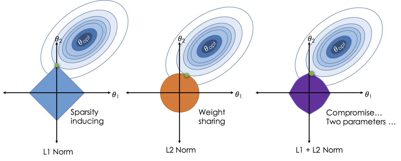
- Dropout is a regularization technique that randomly drops out a fraction of the neurons during training, which can help prevent overfitting and improve generalization.
- Early stopping is a regularization technique that stops the training process when the performance on a validation set starts to degrade, which can help prevent overfitting and improve generalization.
Grief with Gradients
- Vanishing gradients: when the gradients become very small, which can make it difficult for the model to learn and converge.
- This can happen when using activation functions like sigmoid or tanh, which can saturate and lead to very small gradients. To address this issue, we can use activation functions like ReLU or its variants, which do not saturate and can help prevent vanishing gradients.
- The depth of the network can also contribute to vanishing gradients, as the gradients can become smaller as they are propagated back through many layers. To address this issue, we can use techniques like skip connections (e.g., ResNet) or batch normalization, which can help improve the flow of gradients and allow the model to learn more effectively.
- WE can use multi-level hierarchy to allow the model to learn features at different levels of abstraction and train them individually.
- In reinforcement learning, vanishing gradients can also occur when the rewards are sparse or delayed, which can make it difficult for the model to learn from the feedback. To address this issue, we can use techniques like reward shaping, which provides additional rewards to guide the learning process, or we can use algorithms that are designed to handle sparse rewards, such as Proximal Policy Optimization (PPO) or Deep Q-Networks (DQN).
- Exploding gradients: when the gradients become very large, which can cause the model to diverge and fail to converge. This can happen when using activation functions like ReLU, which can lead to large gradients for positive inputs. To address this issue, we can use techniques like gradient clipping, which limits the maximum value of the gradients during training, or we can use activation functions like Leaky ReLU or ELU, which can help prevent exploding gradients by allowing a small slope for negative inputs.
It is often necessary to illustrate the gradient flow during training to diagnose and address issues with vanishing or exploding gradients.
Evaluation
Classification Metrics
Confusion Matrix
A confusion matrix is a table that is used to evaluate the performance of a classification model. It shows the number of true positives, true negatives, false positives, and false negatives, which can be used to compute various evaluation metrics such as accuracy, precision, recall, and F1 score.
Why it is important? For example in a test for a rare disease, we can have 99.9% accuracy by always predicting negative, but this model would be useless for identifying the disease. By looking at the confusion matrix, we can see that the model is not performing well on the positive class and can take steps to improve it, such as collecting more data or using a different algorithm.
| Actual cat | Actual not cat | |
|---|---|---|
| Predicted cat | 50(TP) | 5(FN) |
| Predicted not cat | 10(FP) | 100(TN) |
For multi-class classification problems, the confusion matrix can be extended to show the counts for each class, which can help identify which classes are being misclassified and guide further improvements to the model. Each axe represents the actual and predicted classes, and the values in the matrix represent the counts of true positives, false positives, true negatives, and false negatives for each class. Only the diagonal elements represent the correct predictions, while the off-diagonal elements represent the misclassifications. By analyzing the confusion matrix, we can identify which classes are being confused with each other and take steps to improve the model’s performance on those classes, such as collecting more data or using a different algorithm.
Precision, Recall, F1 Score
- Precision is the ratio of true positives to the total number of predicted positives, which measures the accuracy of the positive predictions. $$Precision = \frac{TP}{TP + FP}$$
- Recall is the ratio of true positives to the total number of actual positives, which measures the ability of the model to identify all positive instances. $$Recall = \frac{TP}{TP + FN}$$
- F1 score is the harmonic mean of precision and recall, which provides a single metric that balances both precision and recall. $$F1\ Score = 2 \cdot \frac{Precision \cdot Recall}{Precision + Recall}$$ F1 score comes from the inverse of the average of the inverses of precision and recall, which is the harmonic mean. It is used to balance the trade-off between precision and recall, especially when there is an imbalance in the classes. A high F1 score indicates that the model has both high precision and high recall, while a low F1 score indicates that the model has either low precision or low recall (or both). It is important to consider both precision and recall when evaluating a classification model, as they can provide different insights into the performance of the model.
- Specificity is the ratio of true negatives to the total number of actual negatives, which measures the ability of the model to identify all negative instances. It is the recall for the negative class, which is also called true negative rate (TNR). $$Specificity = \frac{TN}{TN + FP}$$
- Harmonic mean: $$Harmonic\ Mean = \frac{n}{\sum_{i=1}^{n} \frac{1}{x_i}}$$ This mean is often used when we want to average rates or ratios, such as speeds during a trip or precision and recall in classification problems. It is less affected by extreme values than the arithmetic mean, which can be useful when dealing with imbalanced datasets or when one of the metrics is much lower than the other.
ROC Curve and AUC
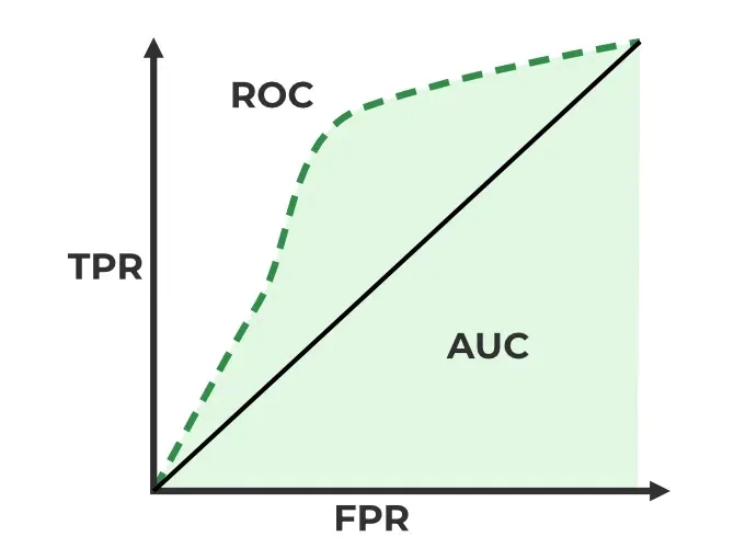
TPR (True Positive Rate) is the ratio of true positives to the total number of actual positives, which measures the ability of the model to identify all positive instances. It is also known as sensitivity or recall. $$TPR = \frac{TP}{TP + FN}$$
False Positive Rate (FPR) is the ratio of false positives to the total number of actual negatives, which measures the rate at which the model incorrectly identifies negative instances as positive. It is calculated as: $$FPR = \frac{FP}{FP + TN}$$
ROC Curve (Receiver Operating Characteristic Curve) is a graphical representation of the performance of a binary classification model as the discrimination threshold is varied. It plots the true positive rate (TPR) against the false positive rate (FPR) at different threshold settings. The TPR is also known as sensitivity or recall, while the FPR is calculated as 1 - specificity. The ROC curve provides a visual way to evaluate the trade-off between sensitivity and specificity for different threshold values.
AUC (Area Under the Curve) is a single scalar value that summarizes the overall performance of a binary classification model based on the ROC curve. It represents the probability that the model will rank a randomly chosen positive instance higher than a randomly chosen negative instance. An AUC of 1 indicates perfect classification, while an AUC of 0.5 indicates random guessing. A higher AUC value indicates better model performance, as it means that the model is better at distinguishing between positive and negative instances across all possible threshold values.
P-R Curve
- Precision-Recall Curve is a graphical representation of the performance of a binary classification model as the discrimination threshold is varied. It plots precision against recall at different threshold settings. The precision-recall curve provides a visual way to evaluate the trade-off between precision and recall for different threshold values, especially in cases where there is an imbalance in the classes. A high area under the precision-recall curve indicates that the model has both high precision and high recall, while a low area indicates that the model has either low precision or low recall (or both).
Regression Metrics
Mean Absolute Error (MAE) is a common evaluation metric for regression problems, which measures the average absolute difference between the predicted and actual values. It is calculated as: $$MAE = \frac{1}{n} \sum_{i=1}^{n} |y_i - \hat{y}_i|$$
RMSE (Root Mean Squared Error) is a common evaluation metric for regression problems, which measures the average magnitude of the errors between the predicted and actual values. It is calculated as the square root of the average of the squared differences between the predicted and actual values. It penalizes larger errors more than smaller errors, which can be useful when we want to give more weight to larger errors. It is calculated as: $$RMSE = \sqrt{\frac{1}{n} \sum_{i=1}^{n} (y_i - \hat{y}_i)^2}$$
R-squared (Coefficient of Determination) is a common evaluation metric for regression problems, which measures the proportion of the variance in the dependent variable that is predictable from the independent variables. It is calculated as:
$$R^2 = 1 - \frac{\sum_{i=1}^n (y_i - \hat{y_i})^2}{\sum_{i=1}^n (y_i - \bar{y})^2}$$
Tuning
Hyperparameter tuning become blows up quickly when we have many hyperparameters to tune, which can make it difficult to find the best combination of hyperparameters for a given model and dataset. Sagemaker provides several tools and techniques for hyperparameter tuning.
hyperparameter tuning jobs
Sagemaker allows you to create hyperparameter tuning jobs. You can specify the range of values for each hyperparameter you care about and the metrics you are optimizing for and Sagemaker will handle the rest. The set of hyperparameters producing the best results can then be deployed as a model. It learns as it goes, so it does’t have to try every possible combination. It will try a few parameters and check whether they have improved the metric. If they have, it will try more parameters in that direction. If they haven’t, it will try parameters in a different direction. This way, it can find the best combination of hyperparameters without having to try every possible combination.
- Take home message: Don’t optimize too many hyperparameters at once, limit the ranges as small a range as possible. Use logarithmic scale when appropriate. Don’t run to many training jobs concurently, This limits how well the process can learn as it goes. Make sure training jobs running on multiple instances report the correct objective metric in the end.
Hyperparameter tuning in AMT
- Early stopping: If a training job is not improving the objective metric after a certain number of epochs, it can be stopped early to save time and resources. Set the
EarlyStoppingTypetoAutoand specify theEarlyStoppingRuleConfigurationto enable early stopping for your hyperparameter tuning job. - Warm Start: Uses one or more previous tuning jobs as a starting point. Inform which hyperparameter combinations to search next can be a way to start where you left off from a stopped hyperparamter job. There are two types of warm start:
IdenticalDataAndAlgorithmandTransferLearning. The former is used when the same dataset and algorithm are used across tuning jobs, while the latter is used when different datasets or algorithms are used but there is some overlap in the hyperparameters being tuned. By using warm start, you can leverage the knowledge gained from previous tuning jobs to improve the efficiency and effectiveness of your hyperparameter tuning process. - Resource limits: You can set limits on the number of training jobs that can run concurrently and the total number of training jobs that can be run for a hyperparameter tuning job. This can help manage resources and prevent excessive costs. You can specify these limits when creating a hyperparameter tuning job by setting the
ResourceLimitsparameter.
Hyperparameter tuning approaches
- Grid Search: This approach involves defining a grid of hyperparameter values and exhaustively evaluating the model for each combination of hyperparameters. While this method can be effective for small hyperparameter spaces, it can become computationally expensive as the number of hyperparameters and their possible values increase.
- Random Search: This approach involves randomly sampling hyperparameter combinations from a defined search space. It can be more efficient than grid search, especially when only a few hyperparameters have a significant impact on the model’s performance. Random search can explore a wider range of hyperparameter values and may find better combinations than grid search in less time. There is no dependence on prior runs, so they can all run in parallel.
- Bayesian Optimization: This approach treats tuning as a regression problem. It learns from each run to coveraage on optimal values. We need to run them sequentially.
- Hyperband: It is appropriate for algorthms that publish results iteratively (like training a neural network over several epochs). It allocates resources dynamically and it can do early stopping and run them in parallel. It is much faster than random search and Bayesian method.
SageMaker Automatic
Autopilot Model Tuning (AMT) SageMaker Automatic Model Tuning (AMT) is a service that helps you to:
- Algorithm selection
- Data preprocessing
- Model tuning
- All infrastructure management I can does all the trial and erro for you, more abrodly, this is called AutoML (Automated Machine Learning).
SageMaker Autopilot workflow:
- load data from s3 for training.
- Select you target column for prediction.
- Automatic model creation.
- Model notebook is available for visisbility and control.
- Model learderboard is available for model comparison.
- Deploy and monitor the best model and refine via notebook if needed.
problem types: binary classification, multi-class classification, regression.
Algorithm Types: Linear Learner, XGBoost, Deep Learning (MLP’s), Ensemble mode.
Input Data: CSV, Parquet.
SageMaker Feature
SageMaker Studio
SageMaker Studio is an integrated development environment (IDE) for machine learning that provides a web-based interface for building, training, and deploying machine learning models. It offers a wide range of tools and features to help data scientists and machine learning engineers streamline their workflow and collaborate more effectively. Some of the key features of SageMaker Studio include:
Jupyter notebooks: SageMaker Studio provides a Jupyter notebook interface that allows you to write and execute code in a web-based environment. You can use Jupyter notebooks to explore your data, build and train machine learning models, and visualize results. It can also can easily switch between hardware configurations.
SageMaker Experiments: This feature allows you to track and compare different machine learning experiments, including the parameters, metrics, and artifacts associated with each experiment. You can use SageMaker Experiments to organize your work and identify the best-performing models.
SageMaker Training Techniques
SageMaker Training Compiler
It is integrated into AWS Deep Learning Containers (DLCs). DLCs are pre-made Docker images for: TensorFlow, PyTorch, MXNet, and Hugging Face. We can use the training compiler by setting enable_sagemaker_training_compiler=True in the estimator. It will then compile & optimize the training jobs on GPU instances. It can accelerate training up to 50%. It convert models into hardware-optimized instructions. It has been tested with Hugging Face Transformers library, etc, and we can also bring our model for testing.
WE need to ensure to use GPU instances. But this is no longer maintained by AWS, so it may not be compatible with the latest versions of the deep learning frameworks.
Warm Pools
It retain and re-use provisioned infrastructure. It is useful if you repeatedly training a model to speed things up. it is used by setting Keep Alive PeriodInSeconds in you training job configuration. It can reduce the startup time for subsequent training jobs by keeping the underlying infrastructure warm and ready to use. This can be particularly beneficial when you have a series of training jobs that need to be run in quick succession, as it can help to minimize the downtime between jobs and improve overall efficiency.
Checkpointing
It creates snapshots during training. We can re-start from these points if necessary or use them for troubleshooting, to analyze the model at different points. It automatically saves checkpoints to Amazon S3 at regular intervals during training. To setup, we can define checkpoint_s3_uri and checkpoint_local_path in the SageMaker Estimator.
Distributed Training
Job parallelism: Run multiple training jobs in parallel. Individual training job parallelism: We have Distributed Data Parallel (DDP) and Distributed Model Parallel (DMP). DDP is used when the model can fit into a single GPU, but we want to speed up training by using multiple GPUs. DMP is used when the model is too large to fit into a single GPU, so we need to split the model across multiple GPUs. Both DDP and DMP can help to speed up training and allow us to train larger models that would not fit on a single GPU. ml.p4d.24xlarge gives us 8 NVIDIA A100 GPUs, which can be used for distributed training.
Sagemaker’s Distributed Training Libraries built on the AWS Custom Collective Library for EC2. It solves a similar problem as MapReduce pr Spark. But it is designed for distribting computation of gradients in gradient descent. There are two main parts:
AIIReduce collective: Distributes computation of gradient updates to/from GPU’s and is implemeted in the SageMaker Distributed Data Parallel (DDP) library. WE need t specify a backend of smdpp to torch.distributed.init_process_group in the traing scripts.
The we need to specify distribution={“smdistributed”: {“dataparallel”: {“enabled”: True}}} in the Pytorch estimator.
AIIGather collective: It manages communication between nodes to improve performance. It offloads communications overhead to the GPU, freeing up GPU’s.
We can also use other distributed Training Libraries. Pytorch DistributedDataParllel (DDP): distribution = {“pytorchddp”: {“enabled”: True}} Torchrun: distribution = {“torch_distributed”: {“enabled”: True}},requires p3, p4, or trn1 instances. DeepSpeed: Open source from Microsoft, for pytorch. Horovod: Open source from Uber, for TensorFlow, Keras, PyTorch, and MXNet.
Sagemaker Model Parallelism Library
A large language model won’t fit on a single machine and we need to distribute the model itself to overcome GPU memory limits.
SageMaker’s interleaved pipelines offers benefits for both Tensorflow and Pytorch.
SageMaker MMP: It goes further. It offers
- optimization state sharding: “Optimization state” is its weights and it requires a stateful optimizer, like Adam.It shards the weights between GPUs. It is generally useful for models with more than 1B parameters.
- Activation checkpointing: Reduces memory usage by clearing activations of certain layers adn recomputing them during a backward pass.
- Activation offloading: Swaps checkpointed activations in a microbatch to/fro CPU.
Use it:
import torch.sagemaker as tsm
tsm.init_process_group(backend="smmp")
It requires a few modifications to the training job launcher object adn it wrap the model and optimizer, slip up the data set. Train with mpi and mpp in the estimator:
estimator = PyTorch(
    ...,
    distribution={
        "smdistributed": {
            "modelparallel": {"enabled": True},
            "dataparallel": {"enabled": True}
        }
    },
)
Sharded Data Parallel (SDP)
It combines parallel data and models. It shards the parameters and also the data. the MPP is there by default in a Deep Learning container for Pytorch.
Elastic Fabric Adapter (EFA)
It is a network device attached to your SageMaker instance. It makes better use of the bandwidth and use with NCCL. MICS (Minimize the communication Scale), This is basicaly another name for what the SageMaker sharded data parallelism provides.