Storage and Data Ingestion
Data types
There are three types of data.
- Structured data and unstructured data. Structured data is organized and can be easily stored in databases.
- Unstructured data is more complex and may require specialized storage solutions. They does not have a predefined structure or scehma. They can be in the form of text, images, videos, audio, etc. Examples of unstructured data include social media posts, customer reviews, and multimedia content. Unstructured data can be more challenging to store and analyze compared to structured data due to its lack of organization and consistency.
- Semi-structured data is a mix of structured and unstructured data. It has some organizational properties but does not conform to a rigid schema. Examples of semi-structured data include JSON, XML, and CSV files, Email headers, log files, etc. Semi-structured data can be easier to store and analyze than unstructured data while still providing flexibility in terms of data representation.
Properties of data
- Volumne: The amount of data being generated and stored as any given time.
- Velocity: The speed at which data is generated, collected and processed.
- Variety: The different types and formats of data being generated, such as structured, unstructured, and semi-structured data.
Data warehouse vs Data lake
Data warehouse is a centralized repository that stores structured data from various sources. Designed for complex queries and analysis. Data is cleaned, transformed, and loaded (ETL process). Typically uses a star or snowflake schema. we use ETL (Extract, Transform, Load) process. It is less agile due to predefined schema. Typically more expensive because of optimizations for complex queries.
Data lake is a storage repository that hodls vast amounts of raw data in tis native format. including structured, semi-structured,and unstructured data. Data is stored in its raw form and can be processed and analyzed using various tools and frameworks. Data lakes are more flexible and scalable than data warehouses, but they may require more effort to manage and maintain. examples of data lake storage solutions include Amazon S3, Azure Data Lake Storage, and Google Cloud Storage, hadoop Distributed File System (HDFS), and Apache Iceberg. We use ELT (Extract, Load, Transform) process.
Data lakehouse is a modern data architecture that combines the best features of data lakes and data warehouses. It provides a unified platform for storing, processing, and analyzing both structured and unstructured data. Data lakehouses use a single storage layer that can handle all types of data, eliminating the need for separate data lakes and data warehouses. They also support ACID transactions, which ensure data consistency and reliability. Examples of data lakehouse solutions include AWS Lake Formation (with S3 and Redshift spectrum). Databricks Lakehouse Platform, Snowflake, and Apache Hudi.
Data Mesh
It is more about governance and organization. Individual teams own “data products” within a given domain. These data products serve various “use cases” around the organization. This called “domain-based data management”. It is Federated governance with central standardsand self-serve data infrastructure.
ETL Pipelines
ETL (Extract, Transform, Load). It’s a process used to move dta from source system into a data warehouse.
- Extract: The first step is to extract data from various source systems, such as databases, APIs, or flat files. This involves connecting to the data sources and retrieving the relevant data.
- Transform: The extracted data is then transformed to fit the target schema of the data warehouse. This may involve cleaning the data, performing calculations, handling missing values, encoding or decoding data (one-hot encoding) and applying business rules to ensure that the data is in a usable format.
- Load: Move the transformed data into the target data warehouse or another data repository. We need to manage ETL pipelines. This process must be automated in some reliable way. Aws Glue is a fully managed ETL service that makes it easy to move data between data stores. There are also orchestration services: EventBridge, Amazon Managed workflows for Apache Airflow. AWS step Functions, AWS Lambda, Glue Workflow, etc.
Data Sources
- JDBC: Java Database Connectivity (JDBC) is a standard API for connecting to relational databases. Plateform-independent and Laguage-independent.
- ODBC: Open Database Connectivity (ODBC) is a standard API for connecting to databases. It is platform-dependent (need drivers) and language-independent, allowing applications to access data from various database management systems (DBMS) using a common interface.
- Raw Logs
- APIs
- Streams
Differnt data formats:
- CSV: Comma-Separated Values (CSV) is a simple file format used to store tabular data, where each line represents a record and each field is separated by a comma. For small to medium-sized datasets, CSV files are easy to create and read. However, they can become inefficient for larger datasets due to their lack of compression and support for complex data types. It is also used for importing and exporting data between different applications and databases.
- Json: Lightweight, text-based, and human-readable dta interchagne format that represnts strutured or semi-structured data based in key-value pairs.
- Avro: Binart format that stores both the data and its schema, allowing it to be processed later with diffent systems without the original system’s context.
- Parquet: Columnar storage format optimized for analytics. Allows for efficient compression and encoding schemes. it is used for analyzing large datasets with analytics engines.Use cases where reading specific columns instead of entire records is benficial. Storing data on distirbuted systems where I/O operations and storage need optimization.
Amazon S3
S3 buckets must have globally unique name (across all regions al accounts). Buckets are defined at the region level. bucket is for storing files.
Each object have a key. The key is the full path:
s3://my-bucket/path/to/my/file.txt
key is the prefix + name and there is not folder structure. S3 is a flat storage system. We can use prefixes to organize objects in a way that resembles a folder structure, but it is not a true hierarchical file system
The maximum size of an object in S3 is 5 TB. If uploading more than 5 GB, we need to use the multipart upload API.
Metadata is alist of text key/valu paris system or use metadata. there are also tags and version ID.
IAM Policies - which API calls should be allowed for a specific user from IAM. S3 bucket policies - Json based policies that define permissions for the entire bucket or specific objects within the bucket.
Versioning
Versioning is a feature in Amazon S3 that allows you to keep multiple versions of an object in the same bucket. When versioning is enabled, each time you upload a new version of an object, S3 assigns it a unique version ID. This allows you to retrieve, restore, or permanently delete specific versions of an object as needed. Versioning provides protection against accidental deletion or overwriting of objects and enables you to maintain a history of changes to your data over time.
Replication
There are two types of replication in S3:
- Cross-Region Replication (CRR): This allows you to automatically replicate objects from one S3 bucket to another bucket in a different AWS region.
- Same-Region Replication (SRR): This allows you to automatically replicate objects from one S3 bucket to another bucket within the same AWS region.
When turn on, only the new objects will be replicated. We can also replicate existing objects by using the S3 Batch Operations feature. For Delete operation, it can replicate delete markers from source to target bucket, but it does not replicate delete operations for existing objects.Deletions with a version ID are not repliacted. There is no “chaining” if replication is enabled on both source and target buckets.
Kinesis Data Streams
Amazon Kinesis Data Streams is a fully managed service that allows you to collect, process, and analyze real-time streaming data at scale. The collected data can be then passed to other AWS services for further processing and analysis as Lambda.
The retention is up to 365 days and it is able to replayed by consumers. Data can not deleted from Kinesis and can has up to 1 MB in size. Each stream is made up of one or more shards, which are the base throughput units of the stream. Each shard can support 1MB/s in and 2MB/s out. Kinesis Producer Library (KPL) is a client library that simplifies the process of producing data to Kinesis Data Streams. KCL is a client library that simplifies the process of consuming data from Kinesis Data Streams.
Data Processing
EMR serverless
EMR (Elastic Map Reduce) Serverless is a serverless big data processing service. We can chose an EMR Release and Runtime (Spark, Hive, Presto, etc.) and submit jobs without having to manage any infrastructure. EMR Serverless automatically provisions and scales the compute resources needed to run the jobs and works, and we can also specify the amount of resources we want to allocate for each job. Clusters will be in one region but across availability zones for high availability. We need to still configure worker nodes.
flowchart LR
IAM["IAM user"]
CLI["AWS CLI(for now)"]
ROLE["Job execution role"]
APP["EMR Serverless Application\n(Spark, Hive, etc.)"]
JOB["EMR Job\n(Spark script,\nHive query...)"]
IAM --> CLI
CLI --> APP
ROLE --> APP
JOB --> APP
%% “Notes” as separate nodes; use <br/> for line breaks and keep text on one line
JOB -.-> JOB_NOTE["aws emr-serverless start-job-run<br/>--application-id <application_id><br/>--execution-role-arn <execution_role_arn><br/>--job-driver ..."]
ROLE -.-> ROLE_NOTE["Allow emr-serverless.amazonaws.com service<br/>S3 access for scripts & data<br/>Glue access (for SparkSQL)<br/>KMS keys as needed"]
classDef note fill:#fff5ad,stroke:#999,color:#000,font-size:11px;
class JOB_NOTE,ROLE_NOTE note;
flow:
- Driver reads your code and creates a logical plan.
- Driver breaks the plan into stages and tasks.
- Executors run the tasks in parallel on worker nodes.
- Executors store intermediate data in memory/disk if needed.
- Executors send results back to the driver.
- Driver aggregates results and completes the job.
Pre-Initialized capacity
For Spark, we add 10% overhead to memory request for drivers adn excutors. we need to make sure that the initial capacity is at least 10% more than requested by the job. Example of creating an EMR Serverless application with Spark runtime and specifying the initial capacity for driver and executor workers:
aws emr-serverless create-application \
  --type "SPARK" \
  --name <"my_application_name"> \
  --release-label "emr-6.5.0-preview" \
  --initial-capacity '{
    "DRIVER": {
      "workerCount": 5,
      "resourceConfiguration": {
        "cpu": "2vCPU",
        "memory": "4GB"
      }
    },
    "EXECUTOR": {
      "workerCount": 50,
      "resourceConfiguration": {
        "cpu": "4vCPU",
        "memory": "8GB"
      }
    }
  }' \
  --maximum-capacity '{
    "cpu": "400vCPU",
    "memory": "1024GB"
  }'
EMR on EKS
Elastic kubernates service, we can use it to run our own kubernates cluster and run our jobs on it.
We can have EMR on EKS, which allows us to run EMR jobs on EKS cluster. Which allows submitting Spark job on Elastic Kubernetes Service without provisioning clusters.
It is fully managed and it allows sharing resources between Spark and other apps on Kubernetes.
Spark
HDFS is a distributed file system designed to run on commodity hardware. Yarn (yet another resource negociator) is a resource management layer for Hadoop that allows multiple applications to share resources in a cluster. MapReduce is a programming model for processing large data sets with a distributed algorithm on a cluster. Spark uses map-reduce but it is more efficient than MapReduce because it can keep data in memory and it has a more flexible programming model.
flowchart TB
    HDFS[HDFS]
    YARN[YARN]
    MR[MapReduce]
    SP[Spark]

    MR --> YARN
    SP --> YARN
    YARN --> HDFS
spark components: Speak Streaming, Spark SQL, Spark MLlib, Spark GraphX, Spark RDD (Resilient Distributed Dataset), Spark Core.
flowchart LR
    DRIVER["Driver Program\n(Spark Context)"]
    CM["Cluster Manager\n(Spark, YARN)"]
    EX1["Executor - Cache - Tasks"]
    EX2["Executor - Cache - Tasks"]
    EX3["Executor - Cache - Tasks"]

    DRIVER --> CM

    CM --> EX1
    CM --> EX2
    CM --> EX3

    DRIVER <--> EX1
    DRIVER <--> EX2
    DRIVER <--> EX3

    EX1 <--> EX2
    EX2 <--> EX3
Spark MLLib
- Classification: logistic regression, naive bayes.
- Rgression
- Decision trees
- Recommemdation engine (ALS)
- Clustering (K-means, Gaussian Mixture)
- LDA (K-Means)
- ML workflow (Pipelines, Cross-validation, Hyperparameter tuning)
- SVD, PCA, statistics
Spark Structured Streaming
Data steams as an unbounded table, we can use SQL to query the data stream. New data is new rows appended to inut table.
Spark Streaming + Kinesis
It can get data from Kinesis stream and process it in real-time. We can use Spark Structured Streaming to read data from Kinesis, perform transformations, and write the results to a sink (e.g., S3, database, etc.). This allows us to build real-time data processing pipelines that can handle high volumes of streaming data.
Zeppelin + spark
It can run spark code interactively (like you can in the spark shell), it can exceute SQL queries against Spark SQL, and it can also visualize the results of the queries. Query results may be visualized in charts and graphs.
Features engineering
Feature engineering is appling our knowledge of the data and the model that we are using to create better features to train your model with. We beed to consider which feature should we use, how to handle missing data, do we need to transform these features in some way? should we create new features from the existing ones?
“Applied machine learning is basically feature engineering” - Andrew Ng. We can’t just throw in raw data and expect good results.
Case
If we have historical data in .csv files and only some of the rows and columns in the files are populated. The columns are not labeled. An ML engineer needs to prepare and store data so that the company can use the data to train ML. we can:
- Use AWS Glue crawlers to infer the schemas and available columns.
- Use AWS Glue DataBrew for data cleaning and feature engineering.
- Store the result back in S3 for training.
The Curse of Dimensionality
Too many feature features can be a problem and with dimension increase, the volume of the space increases exponentially, and the data becomes sparse.
Each feature is a new dimension. We usually use domain knowledge to select features, and we can also use techniques like PCA (Principal Component Analysis). K-eams to reduce the dimensionality of the data while retaining as much variance as possible. We can also use feature selection techniques to select a subset of the most relevant features for our model.
Preparing Data for TF-IDF on Spark and EMR
TF: Term Frequency - how many times a term appears in a document. It is often normalized by the total number of terms in the document to prevent bias towards longer documents. A word that occurs frequently is probably important to that document.
IDF: Inverse Document Frequency - measures how important a term is in the entire corpus. It is calculated as the logarithm (since word frequencies are distributed exponentially and that gives use better weighting of a words overall popularity) of the total number of documents divided by the number of documents containing the term. The idea is that terms that appear in many documents are less informative than those that appear in fewer documents. The words like “the”, “is”, “and” will have high term frequency but they are not important for the meaning of the document, so they will have low IDF. On the other hand, a word like “machine learning” may have a lower term frequency but it is more informative, so it will have a higher IDF.
TF-IDF is the product of TF and IDF, it gives us a weight for each term in each document, which can be used as features for machine learning models. It helps to identify the most important terms in a document and can be used for tasks like text classification, clustering, and information retrieval. TF-IDF assumes a document is just a “bag of words”. Words can be represneted as a has value fir efficiency. Doing this at scale is the hard part and that’s where Spark comes in.
$$ \mathrm{tfidf}(t, d, D) = \mathrm{tf}(t, d) \cdot \mathrm{idf}(t, D) $$
$$ \mathrm{tf}(t,d) = \begin{cases} 1 + \log f_{t,d}, & \text{if } f_{t,d} > 0 \ 0, & \text{if } f_{t,d} = 0 \end{cases} $$
$$ \mathrm{idf}(t, D) = \log!\left(\frac{1 + N}{1 + n_t}\right) + 1 $$
$$ \mathrm{idf}_{\text{prob}}(t, D) = \log!\left(\frac{N - n_t}{n_t}\right) $$
Unigram, bigram, n-gram
An extension of TF-IDF is to not only compute relevency for individual words (unigrams) but also for pairs of words (bigrams) or even longer sequences of words (n-grams). This can capture more context and meaning from the text, as certain phrases may be more informative than individual words. For example, “machine learning” as a bigram may be more informative than “machine” and “learning” as separate unigrams. However, using n-grams can also increase the dimensionality of the feature space, so it’s important to balance the benefits with the computational cost.
A very simple search algorithm could be:
- Compute TF-IDF for every word in a corpus.
- For a given search word, sort the documents by their TF-IDF score for the word.
- Display the result.
AWS Managed AI Services
Aws AI services ar pre-trained ML services for our use case.
flowchart LR

subgraph Generative_AI_Tools
    A["SageMaker JumpStart"]
    B["Amazon Bedrock"]
    C["Amazon Q Business"]
    D["Amazon Q Developer"]
end

subgraph AI_Services

    subgraph Text_and_Documents
        E["Amazon Comprehend"]
        F["Amazon Translate"]
        G["Amazon Textract"]
    end

    subgraph Vision
        H["Amazon Rekognition"]
    end

    subgraph Search
        I["Amazon Kendra"]
    end

    subgraph Chatbots
        J["Amazon Lex"]
    end

    subgraph Speech
        K["Amazon Polly"]
        L["Amazon Transcribe"]
    end

    subgraph Recommendations
        M["Amazon Personalize"]
    end

end

subgraph ML_Platform
    N["Amazon SageMaker"]
end
These services have:
- Responsiveness and Availability: High availability and low latency for end-users.
- Redundancy and Regional Coverage: Deployed across multiple Availability Zones and AWS regions.
- Performance: Specialized CPU and GPUs for specific use-cases for cost saving.
- Token-based Pricing: We pay for what we use, no upfront costs, and can scale as needed.
- Provisioned throughput: For predictable workloads, cost savings and predictable performance.
Amazon Comprehend
It is a fully managed and serverless service for natural language processing - NLP and it uses machine learning to find insights and relationships in text:
- Language of the text
- Extracts key phrases, places, people, brands, or events
- Understands how positive or negative the text is.
- Analyzes text using tokenization and parts of speech.
- Automatically organizes a collection of text files by topic.
Sample use cases:
- Customer feedback analysis: Analyze customer reviews, social media posts, and survey responses to understand customer sentiment and identify common themes.
- Create and groups articles by topics that Comprehend will uncover.
Comprehend - Custom Classification
We can organize documents into categories (classes) that we define. For example, we can categorize customer emails so that we can provide guidance based on the type of the customer request.
It supports different doument types, including plain text, PDF, Word, images, and it can do:
- real-time analysis when new document comes in and treat it synchronously.
- Async Analysis for multiple documents (batch), Asychronous processing for large volumes of documents, and it can take hours to process.
Comprehend - Custom Entity Recognition
- NER - Extracts predefined, general-purpose entites like people, places, organizations, dates, and other standard categories, from text.
- Analyze text for specific terms and noun-based phrases.
- Extract terms like policy numbers, or phrases that imply a customer escalation, anything specific to our business.
- Train the model with custom data such as a list of the entities and documents that contain them.
- This can be real-time or async analysis.
Comprehend - Custom Models
- We can create custom models for entity recognition or document classification. It can be trained on our own data.
- Comprehend manages the model versioning.
- Custom models may be copied between AWS accounts. We can attach IAM policy to a model version, authrizing the other account to use it. The other account can then imports the model. These rules apply:
- The other account must be in same region.
- Need its ARN (identifier of the model), region, and optional KMS key.
- Can be done from the Comprehend console.
Sagemaker and Machine Learning Services
Sagemaker is built to handle the entire machine learning workflow.
graph TD
    A[Deploy model, evaluate results in production] --> B[Train and evaluate a model]
    C[Fetch, clean, prepare data] --> B
    B --> A
    B --> C
For the training and deployment
flowchart TB
    subgraph Client["SageMaker Training & Deployment Client app"]
        A[S3 Training Data]
    end

    subgraph SageMaker["SageMaker"]
        B[Model Training]
    end

    subgraph Deployment["SageMaker Endpoint"]
        C[Model Deployment/Hosting]
        D[SageMaker Endpoint]
    end

    subgraph ECR["ECR"]
        E[Training Code Image]
        F[Inference Code Image]
    end

    subgraph S3["S3"]
        G[S3 Model Artifacts]
    end

    A -->|input| B
    E -->|docker image| B
    B -->|output| G
    G -->|model data| C
    F -->|docker image| C
    C --> D
    Client -.->|invoke| D
All this can be done throught a notebool instance in SageMaker Studio, which is an integrated development environment (IDE) for machine learning.
Data preparation on SageMaker
Data usually comes from S3 and can also ingest from Athena, EMR, Redshift, and Amazon Keyspaces DB.Spark can also be used for data preparation on SageMaker. All the package like sklearn, xgboost, etc. are available in SageMaker. We can also use custom docker images for data preparation.
SageMaker Processing
- Copy data from S3 to the processing container.
- Run the processing script (data cleaning, feature engineering, etc.) inside the container.
- Copy the processed data back to S3 for use in training or other steps in the ML workflow.
Training on SageMaker
Create a training job that specifies the training data location, URL of S3 for training, ML compute resources, Url of S3 bucket for output, ECR path to training code. Training options Built-in training algorithms Spark MLlib TensorFlow / MXNet code PyTorch, Scikit-Learn, RLEstimator / MXNet code XGBoost, Hugging Face, Chainer Your own Docker image Algorithm purchased from AWS marketplace
Deploying Trained Models
Save model to S3 then:
- Persistent endpoint for making individual predictons on demand
- SageMaker Batch Transform to get predictions for an entire dataset.
SageMaker Modes
INput modes
S3 File Mode: copies training data from s3 to local directory in Docker container.
S3 Fast File Mode: SKin to “pipe mode”: Training can begin without waiting to dowload data. Can do random access, but works best with sequential access.
Pipe modeL Streams data directly from S3, mainly replaced by Fast File.
Amazon S3 Express One Zone: High-performance storage class in one AZ, it works with file, fast file, and pipe modes.
Amazon FSx for Lustre: High-performance file system that can be used as a data source for SageMaker training jobs. Scales to 100 GB/s of throughput and millions of IOPS with low latency. In single AZ, rquires VPC (local internet).
Amazon EFS: Requires data to be in EFS (elastic file system) already, requires VPC.
SageMaker’s Built-in Algorithms
Linear Learner
Linear regression and logistic regression for classification and regression tasks. Basically we do fit a line to the training data and do the predictions based on that line.
- RecordIO-wrapped protobuf : Float32 data only.
- CSV: First column assumed to be the label. File and pipe modes supported.
Preprocessing
Training data must be normalized and input data should b shuffled.
Training: Uses stochastic gradient descent (Adam, AdaGrad, SGD, etc), Multiple models are optimized in parallel. Tune L1, L2 regularization.
Validation: Most optimal model is selected.
Hyperparameters
- balance_multiclass_weights: Whether to balance the weights for multiclass classification.
- Learnin_rate, minibatch_size, num_epochs, etc.
- L1 and L2 regularization parameters.
- Weight decay: A regularization technique that adds a penalty to the loss function based on the magnitude of the model’s weights. This helps prevent overfitting by discouraging the model from assigning too much importance to any single feature.
- Target_precision: recall_at_target_precision, the algorithm holds precision at this value while maximizing recall
- Target_recall: precision_at_target_recall, it holds recall at this value while maximizing precision. The algorithm then selects the model that meets the specified criterion: for precision_at_target_recall, it picks the one maximizing precision while holding recall ≥ target_recall; vice versa for recall_at_target_precision. This “tuning-in-training” avoids separate hyperparameter tuning jobs and uses efficient SGD optimizations.
Emsemble methods
Many ensemble methods are based on decision trees, which are a type of model that makes predictions by learning simple decision rules inferred from the data features.
Decision Tree
Decision trees use a greedy, recursive partitioning strategy to find the optimal split at each node. At each step:
- Evaluate all features: The algorithm considers every input variable as a potential splitter
- Find the best split point: For each feature, it tests all possible values to find the threshold that produces the most homogeneous child nodes
- Choose the optimal feature: The feature and split point that maximize purity (or minimize impurity) are selected
Splitting Criteria:
- Classification: Gini impurity, entropy (information gain), misclassification error.
- Regression: Mean squared error (MSE), Sum of squared errors (SSE), Mean absolute error (MAE).
How split points are chosed For Continuous Features The algorithm sorts all unique values of the feature and tests every possible threshold between consecutive values as a potential split point. For a feature with n unique values, there are n−1 candidate split points. The algorithm calculates the impurity reduction for each candidate and selects the threshold that yields the highest purity gain.
For Categorical Features The algorithm evaluates splits based on the categorical values themselves. For a feature with k categories, it considers various ways to partition these categories into two groups (for binary trees).
Gini impurity is calculated as: $$Gini = 1 - \sum_{i=1}^{C} p_i^2$$ where $p_i$ is the proportion of samples belonging to class $i$ in the node, and $C$ is the total number of classes. A lower Gini impurity indicates a more homogeneous node.
Entropy is calculated as: $$Entropy = -\sum_{i=1}^{C} p_i \log_2(p_i)$$ where $p_i$ is the proportion of samples belonging to class $i$ in the node. A lower entropy indicates a more homogeneous node.
Information Gain is calculated as: $$Information\ Gain = Entropy(parent) - \sum_{k=1}^{n} \frac{N_k}{N} Entropy(child_k)$$ where $N$ is the total number of samples in the parent node, $N_k$ is the number of samples in child node $k$, and $n$ is the number of child nodes. The algorithm selects the split that maximizes information gain.
Stop Criteria:
- The recursive splitting continues until a stopping criterion is met.
- The node becomes pure (contains only one class)
- A maximum depth is reached
- The number of samples in a node falls below a minimum threshold
- Further splitting no longer improves predictions significantly
Ensemble learning combines several learners (models) to improve overall performance. The variance of the general model decreases thanks to the bagging technique and the bias of the general model decreases thanks to the boosting technique. Random Forest is a bagging method, while XGBoost and LightGBM are boosting methods.
- Bagging: Bootstrap Aggregating, it trains multiple models on different subsets of the training data and then combines their predictions. It can help reduce variance and prevent overfitting. The selection of subset is done by random sampling with replacement, which means that some data points may be included multiple times in the same subset, while others may not be included at all.
- Boosting: In boosting, models are trained sequentially, with each model trying to correct the errors of the previous one. It can help reduce bias and improve the performance of weak learners. bagging typically involves simple averaging of models, while boosting assigns weights based on accuracy. AdaBoost, Gradient Boosting, XGBoost, and LightGBM are popular boosting algorithms.
Homogeneous vs Heterogeneous Ensembles
- Homogeneous Ensembles: All the models in the ensemble are of the same type. For example, an ensemble of decision trees (Random Forest) or an ensemble of linear models (Linear Learner). But we weight the training data differently for each model, so that each model focuses on different aspects of the data.
- Heterogeneous Ensembles: The models in the ensemble are of different types. For example, an ensemble that combines decision trees, linear models, and neural networks.
XGBoost
eXtreme Gradient Boosting (XGBoost) is an optimized distributed gradient boosting library designed to be highly efficient.
It bosted group of decision trees, new trees made to correct the errors of previous trees. It uses gradient descent to minimize loss as new trees are added.
It can be used both for classification and regression tasks.
Models are serialized and deserialized with pickle.
Hyperparameters
- Subsample: Fraction of the training data to be used for growing each tree. It helps prevent overfitting by introducing randomness into the training process.
- Eta: step size shrinkage used in update to prevents overfitting. After each boosting step, we can directly get the weights of new features, and eta shrinks the feature weights to make the boosting process more conservative.
- Gamma: minimum loss reduction to create a partition; larger means more conservative algorithm.
- Alpha: L1 regularization term on weights. Increasing this value will make the model more conservative.
- Lambda: L2 regularization term on weights. Increasing this value will make the model more conservative.
- eval_metric: Optimize on AUC, error,rmse… if you care about false positives more than accuracy, you might use AUC.
- scale_pos_weight: Adjust balance of positive and negative weights, useful for unbalanced classes. A value greater than 1 will give more weight to the positive class, while a value less than 1 will give more weight to the negative class.
- max_depth: Maximum depth of a tree. Increasing this value will make the model more complex and more likely to overfit. Decreasing this value will make the model simpler and less likely to overfit.
LightGBM
LightGBM is also gradient boosting decision tree algorithm, but it uses a different approach to build trees. It uses Gradient-based One-Side Sampling (GOSS) and Exclusive Feature Bundling (EFB) to speed up the training process and reduce memory usage. GOSS focuses on the instances with larger gradients, while EFB bundles mutually exclusive features together to reduce the number of features. It is more adapt with large datasets and high-dimensional data, and it can be faster than XGBoost in some cases.
It a single or multi-instance CPU algorithm, and it can be used for classification and regression tasks. It is a memory-bound algorithm, M5 EC2 instance is recommended for training.
Hyperparameters
- learning_rate: Similar to eta in XGBoost, it controls the step size shrinkage used in update to prevents overfitting.
- num_leaves: Maximum number of leaves in one tree.
- feasture_fraction: Subset of features to be used for each tree.
- bagging_fraction: Features are randomly sampled to be used for each tree.
- bagging_freq: how often bagging is done.
- max_depth: Maximum depth of a tree.
- min_data_in_leaf: Minimum number of data points in a leaf.
Comparison between XGBoost and LightGBM
Seq2Seq
Input sequence is transformed into a fixed-length vector by an encoder, and then the decoder generates the output sequence from the vector. It is widely used in tasks like machine translation, text summarization, etc. The encoder and decoder can be implemented using RNNs, LSTMs, GRUs, or Transformers.
We need to provide training data, validation data and vocabulary file for seq2seq training. This model an only be trained on single machine but can have multiple GPUs, P3 is adapted for this kind of training.
Hyperparameters
- batch_size: Number of training examples used in one iteration.
- optimiser_type: Adam, sgd, rmsprop, etc.
- num_layers_encoder: Number of layers in the encoder.
- num_layers_decoder: Number of layers in the decoder.
- Can optimize on:
Accuracy (compare to validation dataset): $$\text{Accuracy} = \frac{\text{Number of correct predictions}}{\text{Total number of predictions}}$$
BLEU score (Bilingual Evaluation Understudy): A metric for evaluating the quality of text generated by comparing it to one or more human reference translations. It focuses on precision—how many of the generated n-grams appear in the reference. $$\text{BLEU} = BP \cdot \exp\left(\sum_{n=1}^{N} w_n \log p_n\right)$$ Where $BP$ is the brevity penalty, $w_n$ are the weights for n-grams, and $p_n$ is the precision for n-grams of size $n$. The brevity penalty is calculated as: $$BP = \begin{cases} 1 & \text{if } c > r \ e^{(1 - r/c)} & \text{if } c \leq r \end{cases}$$ where $c$ is the length of the candidate translation and $r$ is the length of the reference translation.
ROUGE score (Recall-Oriented Understudy for Gisting Evaluation): A set of metrics for evaluating automatic summarization and machine translation. It focuses on recall—how many of the reference n-grams appear in the generated text. $$\text{ROUGE-N} = \frac{\sum_{\text{reference summaries}} \sum_{\text{n-grams}} \text{Count}{\text{match}}(\text{n-gram})}{\sum{\text{reference summaries}} \sum_{\text{n-grams}} \text{Count}(\text{n-gram})}$$
Perplexity (Cross-entropy). $$\text{Perplexity} = \exp\left(-\frac{1}{N} \sum_{i=1}^{N} \log P(w_i | w_1 \ldots w_{i-1})\right) = \exp(H)$$
DeepAR
DeepAR is a forecasting algorithm that uses recurrent neural networks (RNNs) to model time series data. It allows us to train the same model over several related time series.
BlazingText
BlazingText is for Text classification and word embedding. It is based on the Word2Vec algorithm, which learns word embeddings by predicting the context of a word given its surrounding words (CBOW) or by predicting a word given its context (Skip-gram) or Batch skip-gram (distributed computation over many CPU nodes). BlazingText can be used for tasks like sentiment analysis, topic classification, etc. It works one single word.
Object2Vec
Like word2vec, but for objects. It learns vector representations of objects based on their co-occurrence in the data. It can be used for tasks like recommendation systems, anomaly detection, etc. It works on objects, which can be users, products, etc.
We can process data into JSON lines and shuffle it.
{"label": "cluster_1", "text": "I love this product!"}
{"label": "cluster_2", "text": "This is the worst experience I've ever had."}
Train with two input channels, two encoders, and a comparator. The encoders can be Average-pooled embeddings, CNN’s, or Birectional LSTM. The comparator is followed by a feed-forward neural network.
Computer vison
SageMaker support frameworks like TensorFlow, PyTorch, MXNet, etc. for computer vision tasks. It also has built-in algorithms like Image Classification and Object Detection. We can also use custom algorithms for computer vision tasks.
Random Cut Forest
Random Cut Forest (RCF) is an algorithm for: Anomaly detection, breaks in peridicity, unclassified data points, and it also attribute anomaly score to each data point.
It creates a forest of trees where each tree is a aprtition of the training data. Then it looks at expected change in complexity of the tree as a result of adding a new data point. The data is sampled randomly and then trained on the sample. RCF can work with Kinesis Analytics for real-time anomaly detection on streaming data.
Hyperparameters
- num_trees: Number of trees in the forest, more trees can reduces noise.
- num_smaples_per_tree: Number of samples used to build each tree, smaller samples can make the model more sensitive to anomalies but also more noisy. 1/num_samples_per_tree approximates the ratio of animalous points to normal data.
Neural Topic Model
Neural Topic Model (NTM) is a topic modeling algorithm that uses neural networks to learn the underlying topics in a collection of documents. It is based on an unsupervised learning algorithm: Neual Variational Inference. It organize documents into topics,and classify or summarize documents based on the topics. We need to define how many topics we want and these topics are a latent representation based on top ranking words.
LDA
Latent Dirichlet Allocation (LDA) is a generative probabilistic model for topic modeling algortihm. It assumes that documents are a mixture of topics and that each topic is a distribution over words. LDA uses a Dirichlet distribution to model the topic distribution for each document and the word distribution for each topic. It is also an unsupervised learning algorithm, and it can be used for tasks like document classification, information retrieval, etc.
Hyperparameters
- num_topics: Number of topics to be extracted from the documents.
- alpha: Hyperparameter for the Dirichlet distribution on the per-document topic distributions. A higher value of alpha leads to more topics being assigned to each document, while a lower value leads to fewer topics being assigned to each document.
KNN
Suppervised learning algorithm for classification and regression tasks. It works by finding the k nearest neighbors of a data point and making predictions based on the majority class (for classification) or the average value (for regression) of those neighbors. It is a non-parametric algorithm, which means it does not make any assumptions about the underlying data distribution. It can be used for tasks like image classification, text classification, etc.
Hyperparameters
- n_neighbors: Number of neighbors to use for making predictions. A smaller value of n_neighbors can lead to a more flexible model that captures local patterns in the data, while a larger value can lead to a smoother model that captures global patterns in the data.
- Sample_size: Number of samples to be used for training the model.
K-Means
Unsupervised learning algorithm for clustering tasks. It divides data into K groups, whre members of a group are as similar as possible to each other. We can define what similar means by defining a distance metric, like Euclidean distance, Manhattan distance, etc. It is an iterative algorithm that starts with K random centroids and then assigns each data point to the nearest centroid, and then updates the centroids based on the mean of the assigned data points. It can be used for tasks like customer segmentation, image segmentation, etc.
Given a dataset:
$$ X = {x_1, x_2, \dots, x_n}, \quad x_i \in \mathbb{R}^d $$
We want to partition the data into $K$ clusters by minimizing the within-cluster sum of squares:
$$ J(\mu, C) = \sum_{k=1}^{K} \sum_{x_i \in C_k} |x_i - \mu_k|^2 $$
Where:
- $C_k$ is the set of points assigned to cluster $k$
- $\mu_k \in \mathbb{R}^d$ is the centroid of cluster $k$
Step1 Initialize centroids:
$$ \mu_1^{(0)}, \mu_2^{(0)}, \dots, \mu_K^{(0)} $$
Step 2 — Repeat Until Convergence
For iteration $t = 1,2,\dots$: $$ C_i^{(t)} = \arg\min_{k \in {1,\dots,K}} |x_i - \mu_k^{(t-1)}|^2 $$
This defines clusters:
$$ C_k^{(t)} = { x_i \mid C_i^{(t)} = k } $$
Recompute centroids as the mean of assigned points:
$$ \mu_k^{(t)} = \frac{1}{|C_k^{(t)}|} \sum_{i : C_i^{(t)} = k} x_i $$
Step 3 — Convergence Criterion Stop if:
$$ \max_k |\mu_k^{(t)} - \mu_k^{(t-1)}| < \varepsilon $$
or if assignments no longer change.
Computational Complexity
Per iteration:
$$ O(n K d) $$
Total complexity:
$$ O(T n K d) $$
Where:
- $n$ = number of samples
- $K$ = number of clusters
- $d$ = dimension
- $T$ = number of iterations
Derivation of the Update Rule
We minimize:
$$ \sum_{x_i \in C_k} |x_i - \mu_k|^2 $$
Take derivative:
$$ \frac{\partial}{\partial \mu_k} \sum_{x_i \in C_k} |x_i - \mu_k|^2 = -2 \sum_{x_i \in C_k} (x_i - \mu_k) $$
Set derivative to zero:
$$ \sum_{x_i \in C_k} (x_i - \mu_k) = 0 $$
Therefore:
$$ \mu_k = \frac{1}{|C_k|} \sum_{x_i \in C_k} x_i $$
PCA
Principal Component Analysis (PCA) is a dimensionality reduction technique that transforms a high-dimensional dataset into a lower-dimensional space while preserving as much variance as possible. It does this by finding the directions (principal components) along which the variance of the data is maximized. PCA can be used for tasks like data visualization, noise reduction, and feature extraction.
The reduced dimensions are called components, and they are the eigenvectors of the covariance matrix of the data. The amount of variance preserved in the reduced space is determined by the eigenvalues corresponding to those eigenvectors. PCA can be used for tasks like data visualization, noise reduction, and feature extraction.
With data, we first create Covariance matrix, then we do the singular value decomposition (SVD) of the covariance matrix to get the eigenvalues and eigenvectors. We then select the top k eigenvectors corresponding to the largest eigenvalues to form the projection matrix.
There are two modes for PCA in SageMaker:
- The regular mode: For sparse data and moderate number of observations and features.
- Randomized: This is used for large number of observations and features. It uses approximate algorithm.
Factorization Machines
Factorization Machines (FM) is a supervised learning algorithm that can model interactions between features in high-dimensional sparse datasets. It is particularly effective for tasks like recommendation systems, click prediction, and regression problems.
The Challenge of Feature Interactions
In many real-world prediction tasks (recommender systems, click-through rate prediction), the input features are:
- High-dimensional: Millions of features after one-hot encoding
- Sparse: Each example has only a few non-zero values
- Rich in interactions: The prediction depends on combinations of features (e.g., user ID × item ID, ad category × page context)
The Problem with Linear Models
A standard linear regression model:
$$ \hat{y}(x) = w_0 + \sum_{i=1}^{d} w_i x_i $$
can only capture the independent effect of each feature. It cannot model that “user A liking item B” is a specific interaction effect.
The Problem with Explicit Interaction Terms
Adding all pairwise interactions naively:
$$ \hat{y}(x) = w_0 + \sum_{i=1}^{d} w_i x_i + \sum_{i=1}^{d}\sum_{j=i+1}^{d} w_{ij} x_i x_j $$
requires $O(d^2)$ parameters. For $d = 1,000,000$ features, this is $10^{12}$ parameters—impossible to estimate, especially since most feature pairs never co-occur in sparse data.
2. The FM Solution: Factorized Interactions
Factorization Machines address this by factorizing the interaction weight $w_{ij}$ into the dot product of two latent vectors $\mathbf{v}_i$ and $\mathbf{v}_j$:
$$ \hat{y}(x) = w_0 + \sum_{i=1}^{d} w_i x_i + \sum_{i=1}^{d}\sum_{j=i+1}^{d} \langle \mathbf{v}_i, \mathbf{v}_j \rangle x_i x_j $$
Components
| Symbol | Description | Dimension |
|---|---|---|
| $w_0$ | Global bias | $\mathbb{R}$ |
| $\mathbf{w}$ | Linear weights | $\mathbb{R}^d$ |
| $\mathbf{V}$ | Embedding matrix | $\mathbb{R}^{d \times k}$ |
| $\mathbf{v}_i$ | Latent vector for feature $i$ | $\mathbb{R}^k$ |
| $k$ | Embedding dimension | $k \ll d$ (typically 10-100) |
Inner Product Definition
$$ \langle \mathbf{v}i, \mathbf{v}j \rangle = \sum{f=1}^{k} v{i,f} \cdot v_{j,f} $$
Key Insight
Instead of learning a unique parameter $w_{ij}$ for each pair (which requires seeing that pair in training), FM learns embeddings $\mathbf{v}_i$ for each feature. The interaction between features $i$ and $j$ is computed as the dot product of their embeddings.
Benefits:
- Parameter reduction: From $O(d^2)$ to $O(dk)$ parameters
- Generalization: Even if features $i$ and $j$ never co-occurred in training, their embeddings can still produce meaningful interactions
3. The Computational Trick: Linear Complexity
Computing all pairwise interactions naively is $O(d^2 k)$—too expensive for high-dimensional sparse data.
The Solution
FM uses an algebraic reformulation to reduce complexity to $O(dk)$:
$$ \sum_{i=1}^{d}\sum_{j=i+1}^{d} \langle \mathbf{v}i, \mathbf{v}j \rangle x_i x_j = \frac{1}{2} \sum{f=1}^{k} \left[ \left(\sum{i=1}^{d} v_{i,f} x_i\right)^2 - \sum_{i=1}^{d} v_{i,f}^2 x_i^2 \right] $$
Why This Works
- Single pass per dimension: The term $\sum_{i=1}^{d} v_{i,f} x_i$ can be computed once per dimension $f$
- Leverages sparsity: For sparse inputs, only non-zero $x_i$ need to be processed
- Linear complexity: The complexity becomes linear in the number of non-zero features
Algorithm Steps
## Pseudocode for FM prediction
def predict(x, w0, w, V, k, d):
    # Linear part
    result = w0
    for i in non_zero_features(x):
        result += w[i] * x[i]

    # Interaction part (O(n*k) where n = non-zero features)
    for f in range(k):
        sum_vf_x = 0
        sum_vf2_x2 = 0
        for i in non_zero_features(x):
            sum_vf_x += V[i, f] * x[i]
            sum_vf2_x2 += (V[i, f] ** 2) * (x[i] ** 2)
        result += 0.5 * (sum_vf_x ** 2 - sum_vf2_x2)

    return result
# Model Training, Tuning, and Evaluation

## Activation Functions

The activation function define the output of a node/neuron given its input signals. It do not participate in the backpropagation process, but it can affect the convergence of the model.

### Binary Step Function
Binary step funciton is either on or off and it can not handle multiple classification abd the vertical slopes don't work well with calculus. It is not used in practice.

### Non-linear Activation Function
Non-linear activation functions are used to introduce non-linearity into the model, which allows it to learn more complex patterns in the data. And grace to it, we can stack multiple layers of neurons to create deep neural networks otherwise the stack of linear layers would still be a linear model.

1. **Sigmoid Function**:
    $$\sigma(x) = \frac{1}{1 + e^{-x}}$$
    (0, 1) range, used for binary classification problems. It can cause vanishing gradient problem when the input is very large or very small.

    Derivative:
    $$\sigma'(x) = \sigma(x)(1 - \sigma(x))$$
2. **Tanh Function**:
    $$\tanh(x) = \frac{e^x - e^{-x}}{e^x + e^{-x}}$$
    (-1, 1) range, zero-centered, used for hidden layers. It can also cause vanishing gradient problem when the input is very large or very small.

    Derivative:
    $$\tanh'(x) = 1 - \tanh^2(x)$$
3. **ReLU Function**:
    $$f(x) = \max(0, x)$$
    Derivative:
    $$f'(x) = \begin{cases} 0 & \text{if }x < 0 \\ 1 & \text{if } x > 0 \end{cases}$$
    Very popular for hidden layers, it can help with the vanishing gradient problem, easy to compute, but it can cause the "dying ReLU" problem where neurons can get stuck in the inactive state and never recover.
4. **Leaky ReLU Function**:
    $$f(x) = \begin{cases} \alpha x & \text{if }x < 0 \\ x & \text{if } x > 0 \end{cases}$$
    Derivative:
    $$f'(x) = \begin{cases} \alpha & \text{if }x < 0 \\ 1 & \text{if } x > 0 \end{cases}$$
    It introduces a small slope for negative inputs, which can help prevent the "dying ReLU" problem and allow the model to learn from negative inputs.
5. Parametric ReLU (PReLU) Function:
    $$f(x) = \begin{cases} \alpha x & \text{if }x < 0 \\ x & \text{if } x > 0 \end{cases}$$
    Derivative:
    $$f'(x) = \begin{cases} \alpha & \text{if }x < 0 \\ 1 & \text{if } x > 0 \end{cases}$$
    Similar to Leaky ReLU, but the slope for negative inputs is learned during training, which can allow the model to adapt to the data and potentially improve performance. here the $\alpha$ is learned parameter.
6. **ELU Function**:
    Exponential Linear Unit (ELU) is defined as:
    $$f(x) = \begin{cases} \alpha (e^x - 1) & \text{if }x < 0 \\ x & \text{if } x > 0 \end{cases}$$
    Derivative:
    $$f'(x) = \begin{cases} f(x) + \alpha & \text{if }x < 0 \\ 1 & \text{if } x > 0 \end{cases}$$
    This one add a exponential component for negative inputs to make the curve smoother.
7. **Swish Function**:
    $$f(x) = x \cdot \sigma(\beta x)$$
    Derivative:
    $$f'(x) = \sigma(\beta x) + \beta x \cdot \sigma(\beta x) \cdot (1 - \sigma(\beta x))$$
    It is a smooth, non-monotonic function that can help improve the performance of deep neural networks, especially in computer vision tasks. It has been shown to outperform ReLU and its variants in some cases.

8. **Maxout**:
    Maxout is a generalization of ReLU that takes the maximum of a set of linear functions. It can be defined as:
    $$f(x) = \max_{i=1}^k (w_i^T x + b_i)$$
    where $w_i$ and $b_i$ are learnable parameters. Maxout can help improve the performance of deep neural networks by allowing them to learn more complex functions, but it can also increase the computational cost and may require more data to train effectively.

9. **Softmax Function**:
    $$\sigma(z)_i = \frac{e^{z_i}}{\sum_{j=1}^K e^{z_j}}$$
    It is used for multi-class classification problems to convert the output of the model into a probability distribution over the classes. But it is not suitable for multi-label classification problems where each instance can belong to multiple classes, because it assumes that the classes are mutually exclusive and the probabilities sum to 1. While sigmoid function can be used for multi-label classification problems, because it can output independent probabilities for each class without the assumption of mutual exclusivity.
## Neural Networks Architectures
### CNN
CNN is a type of neural network that is particularly effective for processing data with a grid-like topology, such as images. It uses convolutional layers to automatically learn spatial hierarchies of features from the input data, which can help improve the performance of the model on tasks like image classification, object detection, and segmentation. CNNs typically consist of multiple **convolutional layers** followed by **pooling layers** and **fully connected layers**. CNN is good to deal with feature-location invariance, but it is not good to deal with rotation and scale variance. To deal with these problems, we can use data augmentation techniques, like random cropping, flipping, rotation, etc. We can also use more advanced architectures, like ResNet, DenseNet, etc.

CNN is inspired by the biological visual cortex, where neurons are organized in a way that allows them to respond to specific regions of the visual field, we called receptive fields which are groups of neurons that only respond to a part of what we see. They receptive fields overlap each other to cover the entire visual field. They feed into higher layers that identify increasingly complex images. For example, some receptive fields identify horizental lines, lines at different angles, etc. These features would feed into a layer that identifies shapes and then might feed into a layer that identifies objects.

For color image, extra layers are needed to process the color channels, which can be done by using 3D convolutional layers that operate on the height, width, and depth (color channels) of the input data. The convolutional layers can learn to extract features from the color channels and combine them to create more complex features that can be used for classification or other tasks.

The structure is typically like this:
```mermaid
graph LR
    A[Input] --> B[Conv]
    B --> C[Pool]
    C --> D[Dropout]
    D --> E[Flatten]
    E --> F[Dense]
    F --> G[Dropout]
    G --> H[Output]
Some common architectures of CNN include LeNet, AlexNet, VGG, ResNet, DenseNet, etc. Each architecture has its own unique features and advantages, and the choice of architecture depends on the specific task and dataset being used. Resnet is the deepest one with skip connections that can help with the vanishing gradient problem and allow the model to learn more complex features.
Recurrent Neural Networks (RNNs)
RNNs are a type of neural network that is designed to process sequential data, such as time series, natural language, etc. It can deal with with data of arbitrary length. They use recurrent connections to allow information to persist across time steps, which can help the model learn patterns in the data that depend on previous inputs. RNNs typically consist of a hidden state that is updated at each time step based on the current input and the previous hidden state. However, RNNs can suffer from the vanishing gradient problem when processing long sequences, which can make it difficult for the model to learn long-term dependencies in the data. To address this issue, more advanced architectures like Long Short-Term Memory (LSTM) and Gated Recurrent Units (GRU) have been developed, which use gating mechanisms to control the flow of information and allow the model to learn long-term dependencies more effectively.
flowchart LR
    subgraph RNN_Node["RNN node (time t)"]
        direction LR

        %% Inputs
        X["x_t"]
        H_prev["h_{t-1}"]

        %% Concatenation
        CAT["concat"]

        %% Linear Transformation
        LIN["W · [x_t, h_{t-1}] + b"]

        %% Activation
        TANH["tanh"]

        %% Output
        H_curr["h_t"]
    end

    %% Feedback loop
    H_curr -.->|next step| H_prev

    %% Flow
    X --> CAT
    H_prev --> CAT
    CAT --> LIN --> TANH --> H_curr
We can also have multiple cells of RNNs to process the sequence, which is called stacked RNNs. We can also have bidirectional RNNs that process the sequence in both forward and backward directions to capture information from both past and future inputs.
The RNNs can do sequence-to-sequence learning, squence to vector learning, vector to sequence learning and also sequence to vector then vector to sequence learning which is called encoder-decoder architecture.
We train RNN. We can use backpropagation through time (BPTT) to train RNNs, which is a variant of backpropagation that takes into account the sequential nature of the data. During training, we unroll the RNN for a certain number of time steps and compute the loss at each time step. We then backpropagate the gradients through the unrolled network to update the weights. However, BPTT can be computationally expensive and may not be suitable for very long sequences. To address this issue, truncated BPTT can be used, which limits the number of time steps that are unrolled during training.
BPTT loop (full sequence):
- Forward: run through all unrolled steps, cache activations.
- Backward through time: start from the loss at the end, propagate gradients step by step to the start. Each step contributes a gradient to the same weight tensors.
- Accumulate: sum (or average) those per-step gradients for each shared weight.
- Optimizer step: apply one update (e.g., SGD/Adam) to the shared weights.
Truncated BPTT:
- Unroll K steps, backprop over those K, update weights.
- Move the window forward (carry the hidden state), repeat. Gradients only flow within each window, but weights keep getting updated, so information from distant timesteps influences learning across windows.
LSTM
LSTM is a type of RNN that is designed to address the vanishing gradient problem and allow the model to learn long-term dependencies in the data. It uses a gating mechanism to control the flow of information through the network, which allows it to selectively remember or forget information from previous time steps. The LSTM architecture consists of three main components: the input gate, the forget gate, and the output gate.
flowchart LR

    %% External inputs / outputs
    Ct_prev["C_t-1"]
    ht_prev["h_t-1"]
    xt["x_t"]

    ht["h_t"]
    Ct_out["C_t"]

    %% LSTM cell
    subgraph CELL["LSTM cell at time t"]
        direction LR

        %% Shared input to all gates: (x_t, h_t-1)
        XH["(x_t, h_t-1)"]

        %% Gate MLPs
        F_sigma["sigma (forget gate)"]
        I_sigma["sigma (input gate)"]
        C_cand_tanh["tanh (candidate)"]
        O_sigma["sigma (output gate)"]

        f_t["f_t"]
        i_t["i_t"]
        C_cand["C_t_tilde"]
        o_t["o_t"]

        %% Cell state operations
        F_mul["*  (f_t * C_t-1)"]
        I_mul["*  (i_t * C_t_tilde)"]
        C_add["+  (sum)"]
        Ct["C_t"]
        TanhCt["tanh(C_t)"]
        H_mul["*  (o_t * tanh(C_t))"]

        %% Fan-out of (x_t, h_t-1) to all gates
        XH --> F_sigma --> f_t
        XH --> I_sigma --> i_t
        XH --> C_cand_tanh --> C_cand
        XH --> O_sigma --> o_t

        %% Top cell-state line and gating
        Ct_prev --> F_mul
        f_t --> F_mul

        C_cand --> I_mul
        i_t --> I_mul

        F_mul --> C_add
        I_mul --> C_add
        C_add --> Ct
        Ct --> TanhCt --> H_mul
        o_t --> H_mul
    end

    %% Connect external nodes to cell
    ht_prev --> XH
    xt --> XH

    H_mul --> ht
    Ct --> Ct_out
GRU
GRU is a type of RNN that is similar to LSTM but has a simpler architecture. It uses two gates, the update gate and the reset gate, to control the flow of information through the network. The update gate determines how much of the previous hidden state should be retained, while the reset gate determines how much of the previous hidden state should be ignored.
Transformer
Transformer is a type of neural network architecture that is designed to process sequential data, such as natural, there is a blog that explain this one. Transformer.
Tuning
Neural networks are trained using SDG or its variants, like Adam, RMSProp, etc. The training process involves updating the weights of the model based on the gradients computed from the loss function. The choice of optimizer can affect the convergence and performance of the model. It is important to experiment with different optimizers and learning rates to find the best combination for your specific problem.
Learning Rate
Learning rate is a hyperparameter that controls the step size at each iteration while moving toward a minimum of the loss function. A learning rate that is too high can cause the model to diverge, while a learning rate that is too low can cause the model to converge very slowly. It is important to find the right learning rate for your specific problem, which can be done through experimentation and techniques like learning rate schedules or adaptive learning rates.
Batch size
Batch size is the number of training examples used in one iteration of training. A smaller batch size can lead to a more noisy gradient estimate, which can help the model escape local minima and potentially improve generalization. However, it can also lead to slower convergence and may require more iterations to reach a good solution. A larger batch size can provide a more accurate gradient estimate, which can lead to faster convergence, but it may also cause the model to get stuck in local minima and may require more memory to train effectively. It is important to experiment with different batch sizes to find the best one for your specific problem. Random shuffling at each epoch can make the training more robust and help the model generalize better to unseen data and we got very inconsistent results from run to run.
Optimizer
The choice of optimizer can affect the convergence and performance of the model. Some common optimizers include Stochastic Gradient Descent (SGD), Adam, RMSProp, etc. Each optimizer has its own advantages and disadvantages, and the best choice depends on the specific problem and dataset being used. It is important to experiment with different optimizers to find the best one for your specific problem.
Regularization
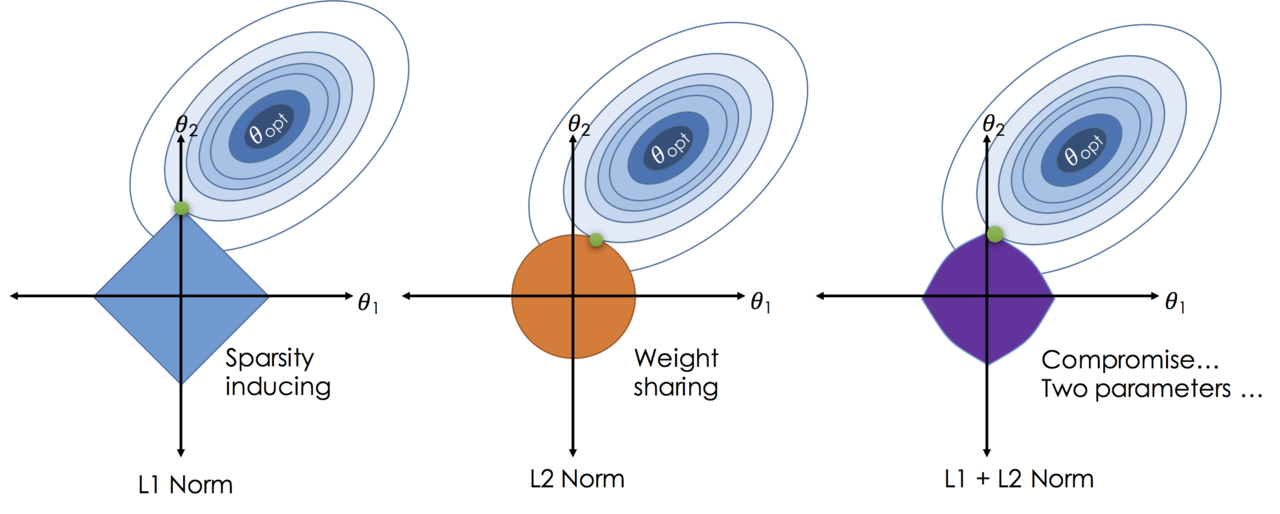
Regularization is a technique used to prevent overfitting in machine learning models. It works by adding a penalty term to the loss function that discourages the model from fitting the training data too closely. Some common regularization techniques include L1 regularization, L2 regularization, dropout, early stopping etc. Each regularization technique has its own advantages and disadvantages, and the best choice depends on the specific problem and dataset being used. It is important to experiment with different regularization techniques to find the best one for your specific problem.
- L1 regularization adds a penalty term to the loss function that is proportional to the absolute value of the weights, which can encourage sparsity in the model and lead to feature selection. $$L1\ regularization: \lambda \sum_{i} |w_i|$$ This is also called Lasso regression in linear regression, it can lead to some weights being exactly zero, which can help with feature selection and interpretability of the model. However, it can also lead to a less stable model and may not perform well when there are many correlated features.
- L2 regularization adds a penalty term to the loss function that is proportional to the square of the weights, which can encourage smaller weights and lead to a more stable model. $$L2\ regularization: \lambda \sum_{i} w_i^2$$ This is also called Ridge regression in linear regression, it can help prevent overfitting by discouraging large weights, but it does not lead to sparsity and may not perform well when there are many irrelevant features.
- Dropout is a regularization technique that randomly drops out a fraction of the neurons during training, which can help prevent overfitting and improve generalization.
- Early stopping is a regularization technique that stops the training process when the performance on a validation set starts to degrade, which can help prevent overfitting and improve generalization.
Grief with Gradients
- Vanishing gradients: when the gradients become very small, which can make it difficult for the model to learn and converge.
- This can happen when using activation functions like sigmoid or tanh, which can saturate and lead to very small gradients. To address this issue, we can use activation functions like ReLU or its variants, which do not saturate and can help prevent vanishing gradients.
- The depth of the network can also contribute to vanishing gradients, as the gradients can become smaller as they are propagated back through many layers. To address this issue, we can use techniques like skip connections (e.g., ResNet) or batch normalization, which can help improve the flow of gradients and allow the model to learn more effectively.
- WE can use multi-level hierarchy to allow the model to learn features at different levels of abstraction and train them individually.
- In reinforcement learning, vanishing gradients can also occur when the rewards are sparse or delayed, which can make it difficult for the model to learn from the feedback. To address this issue, we can use techniques like reward shaping, which provides additional rewards to guide the learning process, or we can use algorithms that are designed to handle sparse rewards, such as Proximal Policy Optimization (PPO) or Deep Q-Networks (DQN).
- Exploding gradients: when the gradients become very large, which can cause the model to diverge and fail to converge. This can happen when using activation functions like ReLU, which can lead to large gradients for positive inputs. To address this issue, we can use techniques like gradient clipping, which limits the maximum value of the gradients during training, or we can use activation functions like Leaky ReLU or ELU, which can help prevent exploding gradients by allowing a small slope for negative inputs.
It is often necessary to illustrate the gradient flow during training to diagnose and address issues with vanishing or exploding gradients.
Evaluation
Classification Metrics
Confusion Matrix
A confusion matrix is a table that is used to evaluate the performance of a classification model. It shows the number of true positives, true negatives, false positives, and false negatives, which can be used to compute various evaluation metrics such as accuracy, precision, recall, and F1 score.
Why it is important? For example in a test for a rare disease, we can have 99.9% accuracy by always predicting negative, but this model would be useless for identifying the disease. By looking at the confusion matrix, we can see that the model is not performing well on the positive class and can take steps to improve it, such as collecting more data or using a different algorithm.
| Actual cat | Actual not cat | |
|---|---|---|
| Predicted cat | 50(TP) | 5(FN) |
| Predicted not cat | 10(FP) | 100(TN) |
For multi-class classification problems, the confusion matrix can be extended to show the counts for each class, which can help identify which classes are being misclassified and guide further improvements to the model. Each axe represents the actual and predicted classes, and the values in the matrix represent the counts of true positives, false positives, true negatives, and false negatives for each class. Only the diagonal elements represent the correct predictions, while the off-diagonal elements represent the misclassifications. By analyzing the confusion matrix, we can identify which classes are being confused with each other and take steps to improve the model’s performance on those classes, such as collecting more data or using a different algorithm.
Precision, Recall, F1 Score
- Precision is the ratio of true positives to the total number of predicted positives, which measures the accuracy of the positive predictions. $$Precision = \frac{TP}{TP + FP}$$
- Recall is the ratio of true positives to the total number of actual positives, which measures the ability of the model to identify all positive instances. $$Recall = \frac{TP}{TP + FN}$$
- F1 score is the harmonic mean of precision and recall, which provides a single metric that balances both precision and recall. $$F1\ Score = 2 \cdot \frac{Precision \cdot Recall}{Precision + Recall}$$ F1 score comes from the inverse of the average of the inverses of precision and recall, which is the harmonic mean. It is used to balance the trade-off between precision and recall, especially when there is an imbalance in the classes. A high F1 score indicates that the model has both high precision and high recall, while a low F1 score indicates that the model has either low precision or low recall (or both). It is important to consider both precision and recall when evaluating a classification model, as they can provide different insights into the performance of the model.
- Specificity is the ratio of true negatives to the total number of actual negatives, which measures the ability of the model to identify all negative instances. It is the recall for the negative class, which is also called true negative rate (TNR). $$Specificity = \frac{TN}{TN + FP}$$
- Harmonic mean: $$Harmonic\ Mean = \frac{n}{\sum_{i=1}^{n} \frac{1}{x_i}}$$ This mean is often used when we want to average rates or ratios, such as speeds during a trip or precision and recall in classification problems. It is less affected by extreme values than the arithmetic mean, which can be useful when dealing with imbalanced datasets or when one of the metrics is much lower than the other.
ROC Curve and AUC
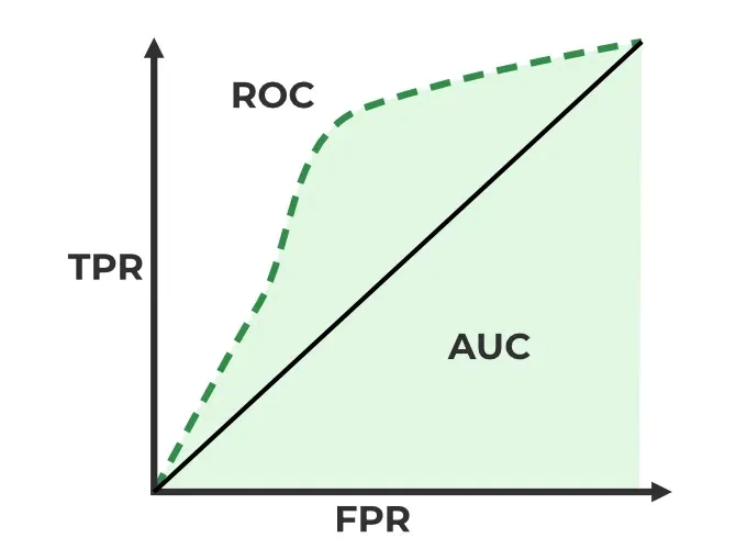
TPR (True Positive Rate) is the ratio of true positives to the total number of actual positives, which measures the ability of the model to identify all positive instances. It is also known as sensitivity or recall. $$TPR = \frac{TP}{TP + FN}$$
False Positive Rate (FPR) is the ratio of false positives to the total number of actual negatives, which measures the rate at which the model incorrectly identifies negative instances as positive. It is calculated as: $$FPR = \frac{FP}{FP + TN}$$
ROC Curve (Receiver Operating Characteristic Curve) is a graphical representation of the performance of a binary classification model as the discrimination threshold is varied. It plots the true positive rate (TPR) against the false positive rate (FPR) at different threshold settings. The TPR is also known as sensitivity or recall, while the FPR is calculated as 1 - specificity. The ROC curve provides a visual way to evaluate the trade-off between sensitivity and specificity for different threshold values.
AUC (Area Under the Curve) is a single scalar value that summarizes the overall performance of a binary classification model based on the ROC curve. It represents the probability that the model will rank a randomly chosen positive instance higher than a randomly chosen negative instance. An AUC of 1 indicates perfect classification, while an AUC of 0.5 indicates random guessing. A higher AUC value indicates better model performance, as it means that the model is better at distinguishing between positive and negative instances across all possible threshold values.
P-R Curve
- Precision-Recall Curve is a graphical representation of the performance of a binary classification model as the discrimination threshold is varied. It plots precision against recall at different threshold settings. The precision-recall curve provides a visual way to evaluate the trade-off between precision and recall for different threshold values, especially in cases where there is an imbalance in the classes. A high area under the precision-recall curve indicates that the model has both high precision and high recall, while a low area indicates that the model has either low precision or low recall (or both).
Regression Metrics
Mean Absolute Error (MAE) is a common evaluation metric for regression problems, which measures the average absolute difference between the predicted and actual values. It is calculated as: $$MAE = \frac{1}{n} \sum_{i=1}^{n} |y_i - \hat{y}_i|$$
RMSE (Root Mean Squared Error) is a common evaluation metric for regression problems, which measures the average magnitude of the errors between the predicted and actual values. It is calculated as the square root of the average of the squared differences between the predicted and actual values. It penalizes larger errors more than smaller errors, which can be useful when we want to give more weight to larger errors. It is calculated as: $$RMSE = \sqrt{\frac{1}{n} \sum_{i=1}^{n} (y_i - \hat{y}_i)^2}$$
R-squared (Coefficient of Determination) is a common evaluation metric for regression problems, which measures the proportion of the variance in the dependent variable that is predictable from the independent variables. It is calculated as:
$$R^2 = 1 - \frac{\sum_{i=1}^n (y_i - \hat{y_i})^2}{\sum_{i=1}^n (y_i - \bar{y})^2}$$
Tuning
Hyperparameter tuning become blows up quickly when we have many hyperparameters to tune, which can make it difficult to find the best combination of hyperparameters for a given model and dataset. Sagemaker provides several tools and techniques for hyperparameter tuning.
hyperparameter tuning jobs
Sagemaker allows you to create hyperparameter tuning jobs. You can specify the range of values for each hyperparameter you care about and the metrics you are optimizing for and Sagemaker will handle the rest. The set of hyperparameters producing the best results can then be deployed as a model. It learns as it goes, so it does’t have to try every possible combination. It will try a few parameters and check whether they have improved the metric. If they have, it will try more parameters in that direction. If they haven’t, it will try parameters in a different direction. This way, it can find the best combination of hyperparameters without having to try every possible combination.
- Take home message: Don’t optimize too many hyperparameters at once, limit the ranges as small a range as possible. Use logarithmic scale when appropriate. Don’t run to many training jobs concurently, This limits how well the process can learn as it goes. Make sure training jobs running on multiple instances report the correct objective metric in the end.
Hyperparameter tuning in AMT
- Early stopping: If a training job is not improving the objective metric after a certain number of epochs, it can be stopped early to save time and resources. Set the
EarlyStoppingTypetoAutoand specify theEarlyStoppingRuleConfigurationto enable early stopping for your hyperparameter tuning job. - Warm Start: Uses one or more previous tuning jobs as a starting point. Inform which hyperparameter combinations to search next can be a way to start where you left off from a stopped hyperparamter job. There are two types of warm start:
IdenticalDataAndAlgorithmandTransferLearning. The former is used when the same dataset and algorithm are used across tuning jobs, while the latter is used when different datasets or algorithms are used but there is some overlap in the hyperparameters being tuned. By using warm start, you can leverage the knowledge gained from previous tuning jobs to improve the efficiency and effectiveness of your hyperparameter tuning process. - Resource limits: You can set limits on the number of training jobs that can run concurrently and the total number of training jobs that can be run for a hyperparameter tuning job. This can help manage resources and prevent excessive costs. You can specify these limits when creating a hyperparameter tuning job by setting the
ResourceLimitsparameter.
Hyperparameter tuning approaches
- Grid Search: This approach involves defining a grid of hyperparameter values and exhaustively evaluating the model for each combination of hyperparameters. While this method can be effective for small hyperparameter spaces, it can become computationally expensive as the number of hyperparameters and their possible values increase.
- Random Search: This approach involves randomly sampling hyperparameter combinations from a defined search space. It can be more efficient than grid search, especially when only a few hyperparameters have a significant impact on the model’s performance. Random search can explore a wider range of hyperparameter values and may find better combinations than grid search in less time. There is no dependence on prior runs, so they can all run in parallel.
- Bayesian Optimization: This approach treats tuning as a regression problem. It learns from each run to coveraage on optimal values. We need to run them sequentially.
- Hyperband: It is appropriate for algorthms that publish results iteratively (like training a neural network over several epochs). It allocates resources dynamically and it can do early stopping and run them in parallel. It is much faster than random search and Bayesian method.
SageMaker Automatic
Autopilot Model Tuning (AMT) SageMaker Automatic Model Tuning (AMT) is a service that helps you to:
- Algorithm selection
- Data preprocessing
- Model tuning
- All infrastructure management I can does all the trial and erro for you, more abrodly, this is called AutoML (Automated Machine Learning).
SageMaker Autopilot workflow:
- load data from s3 for training.
- Select you target column for prediction.
- Automatic model creation.
- Model notebook is available for visisbility and control.
- Model learderboard is available for model comparison.
- Deploy and monitor the best model and refine via notebook if needed.
problem types: binary classification, multi-class classification, regression.
Algorithm Types: Linear Learner, XGBoost, Deep Learning (MLP’s), Ensemble mode.
Input Data: CSV, Parquet.
SageMaker Feature
SageMaker Studio
SageMaker Studio is an integrated development environment (IDE) for machine learning that provides a web-based interface for building, training, and deploying machine learning models. It offers a wide range of tools and features to help data scientists and machine learning engineers streamline their workflow and collaborate more effectively. Some of the key features of SageMaker Studio include:
Jupyter notebooks: SageMaker Studio provides a Jupyter notebook interface that allows you to write and execute code in a web-based environment. You can use Jupyter notebooks to explore your data, build and train machine learning models, and visualize results. It can also can easily switch between hardware configurations.
SageMaker Experiments: This feature allows you to track and compare different machine learning experiments, including the parameters, metrics, and artifacts associated with each experiment. You can use SageMaker Experiments to organize your work and identify the best-performing models.
SageMaker Training Techniques
SageMaker Training Compiler
It is integrated into AWS Deep Learning Containers (DLCs). DLCs are pre-made Docker images for: TensorFlow, PyTorch, MXNet, and Hugging Face. We can use the training compiler by setting enable_sagemaker_training_compiler=True in the estimator. It will then compile & optimize the training jobs on GPU instances. It can accelerate training up to 50%. It convert models into hardware-optimized instructions. It has been tested with Hugging Face Transformers library, etc, and we can also bring our model for testing.
WE need to ensure to use GPU instances. But this is no longer maintained by AWS, so it may not be compatible with the latest versions of the deep learning frameworks.
Warm Pools
It retain and re-use provisioned infrastructure. It is useful if you repeatedly training a model to speed things up. it is used by setting Keep Alive PeriodInSeconds in you training job configuration. It can reduce the startup time for subsequent training jobs by keeping the underlying infrastructure warm and ready to use. This can be particularly beneficial when you have a series of training jobs that need to be run in quick succession, as it can help to minimize the downtime between jobs and improve overall efficiency.
This process eliminates the overhead of resource provisioning, container pull, and environment initialization for subsequent runs. This directly minimizes infrastructure startup time as required, and maintains the required security isolation as warm pool resources are not shared with other AWS customers.
Checkpointing
It creates snapshots during training. We can re-start from these points if necessary or use them for troubleshooting, to analyze the model at different points. It automatically saves checkpoints to Amazon S3 at regular intervals during training. To setup, we can define checkpoint_s3_uri and checkpoint_local_path in the SageMaker Estimator.
Distributed Training
Job parallelism: Run multiple training jobs in parallel. Individual training job parallelism: We have Distributed Data Parallel (DDP) and Distributed Model Parallel (DMP). DDP is used when the model can fit into a single GPU, but we want to speed up training by using multiple GPUs. DMP is used when the model is too large to fit into a single GPU, so we need to split the model across multiple GPUs. Both DDP and DMP can help to speed up training and allow us to train larger models that would not fit on a single GPU. ml.p4d.24xlarge gives us 8 NVIDIA A100 GPUs, which can be used for distributed training.
Sagemaker’s Distributed Training Libraries built on the AWS Custom Collective Library for EC2. It solves a similar problem as MapReduce pr Spark. But it is designed for distribting computation of gradients in gradient descent. There are two main parts:
AIIReduce collective: Distributes computation of gradient updates to/from GPU’s and is implemeted in the SageMaker Distributed Data Parallel (DDP) library. WE need t specify a backend of smdpp to torch.distributed.init_process_group in the traing scripts.
The we need to specify distribution={“smdistributed”: {“dataparallel”: {“enabled”: True}}} in the Pytorch estimator.
AIIGather collective: It manages communication between nodes to improve performance. It offloads communications overhead to the GPU, freeing up GPU’s.
We can also use other distributed Training Libraries. Pytorch DistributedDataParllel (DDP): distribution = {“pytorchddp”: {“enabled”: True}} Torchrun: distribution = {“torch_distributed”: {“enabled”: True}},requires p3, p4, or trn1 instances. DeepSpeed: Open source from Microsoft, for pytorch. Horovod: Open source from Uber, for TensorFlow, Keras, PyTorch, and MXNet.
Sagemaker Model Parallelism Library
A large language model won’t fit on a single machine and we need to distribute the model itself to overcome GPU memory limits.
SageMaker’s interleaved pipelines offers benefits for both Tensorflow and Pytorch.
SageMaker MMP: It goes further. It offers
- optimization state sharding: “Optimization state” is its weights and it requires a stateful optimizer, like Adam.It shards the weights between GPUs. It is generally useful for models with more than 1B parameters.
- Activation checkpointing: Reduces memory usage by clearing activations of certain layers adn recomputing them during a backward pass.
- Activation offloading: Swaps checkpointed activations in a microbatch to/fro CPU.
Use it:
import torch.sagemaker as tsm
tsm.init_process_group(backend="smmp")
It requires a few modifications to the training job launcher object adn it wrap the model and optimizer, slip up the data set. Train with mpi and mpp in the estimator:
estimator = PyTorch(
    ...,
    distribution={
        "smdistributed": {
            "modelparallel": {"enabled": True},
            "dataparallel": {"enabled": True}
        }
    },
)
Sharded Data Parallel (SDP)
It combines parallel data and models. It shards the parameters and also the data. the MPP is there by default in a Deep Learning container for Pytorch.
Elastic Fabric Adapter (EFA)
It is a network device attached to your SageMaker instance. It makes better use of the bandwidth and use with NCCL. MICS (Minimize the communication Scale), This is basicaly another name for what the SageMaker sharded data parallelism provides.
Application of Transformers
Some Terms for LLMs:
- Foundation Models: Large pre-trained models that can be fine-tuned for specific tasks. Examples include GPT-3, BERT, and T5.
- Tokens: Numerical respresentations of words or parts of wrods.
- embeddings: Dense vector representations of tokens that capture their semantic meaning.
- Top-p sampling: Threshold probability for token inclusion. higher -> more random.
- Top-k sampling: K candidates with highest probabilities are considered for sampling. higher -> more random.
- Temperature: The level of randomness in selecting the next word in the output from those tokens.
- Context window: The number of tokens the model can consider at once. Longer context windows allow for more coherent and contextually relevant responses.
- Max tokens: Limit for total number of tokens for input or output.
Transfer Learning (Fine-tuning) with Transformers
- We add additional training data throught the whole thing.
- We often freeze specific layers and re-train others: Train a new tokenizer to learn a new language.
- Add a layer on top of the pre-trained model:
- A few layer may be all that’s needed.
- Provide examples of prompts and desired completions.
- Adapt it to classification or otehr tasks.
Bedrock
The bedrock of generative AI applications. It provides access to foundation models, retrieval augmented generation (RAG), knowledge bases, vector stores, guardrails, and LLM agents. With Bedrock, you can build and deploy generative AI applications quickly and easily without having to manage the underlying infrastructure.
- Bedrock: Manage, deploy, and train models.
- Bedrock-runtime: Perform inference (execute prompts, generate embeddings, etc.) against these models. It provides Converse, converseStream, InvokeModel, and InvokeModelStream APIs.
- bedrock-agent: It manage, deploy, train LLM agents and knowledge bases.
- bedrock-agent-runtime: It performs inference against agents and knowledge bases, It has InvokeAgent, Retrieve, RetrieveAndGenerate APIs.
Bedrock IAM permissions: It must use with an IAM user (not root), User must have permissions to use Bedrock and the underlying models.
Fune tuning with Bedrock
Fune tuning
Bedrock provides a simple and efficient way to fine-tune foundation models for specific tasks. You can use the Bedrock API to fine-tune a model on your own dataset, and then use the fine-tuned model for inference. This allows you to customize the behavior of the model to better suit your specific use case. The train data must be in JSONL format, where each line is a JSON object representing a training example. The JSON object should have the following structure:
{
  "input": "The input text for the model.",
  "output": "The desired output text for the model."
}
You can put them on the S3 and provide the S3 URI to the Bedrock API when fine-tuning the model. Bedrock will then use this data to fine-tune the model and improve its performance on your specific task.
Continued Pre-Training
It is like fine-tuning, but instead of training the model on a specific task, you train it on a larger dataset that is more relevant to your use case. This can help the model learn more about the specific domain or language you are working with. It is unlabeled data, so you don’t need to provide input-output pairs.
Retrival Augmented Generation (RAG)
upload documents to s3 and other source like webcrawler, confluence, salesforce, sharepoint into Bedrock knowledge base. Chose the embedding model and dimension and a store serveing like Amazon OpenSearch. Then We can use agent system or Rag from Amazon Bedrock to retrieve relevant information from the knowledge base and generate responses based on that information.
Amazon Bedrock Guardrails
Content filtering for prompts and responses. It works with text foundation models, word filtering, topic filtering, profanities, PII removal (or masking).
- contextual grounding check: It helps prevent hallucination and measures “grounding” (how similar the response is to the contextual data received) and relevance (of reponse to the query). It can filter out responses that are not grounded or relevant.
- We can configure the “blocked message response”.
We can add a bedrock guardrail from bedrock and define these rules as pro
Tools and agents
In Bedrock, the tools can be Lambda functions, and we need prompt engineering to use them. The model decompose the promblem into subproblems, and then call action groups, knowledge bases, and tools to solve the subproblems. An action group is a collection of tools.
MLOps with AWS
Deployment Safeguards
Deployment Guardrails are for synchronous or real-time inference endpoints. It can control shifting traffic to new models and Auto-rollbacls.
- Canary deployment: It is a deployment strategy that gradually rolls out new changes to a small subset of users before making it available to the entire user base. This allows us to monitor the performance and behavior of the new changes in a controlled environment and quickly roll back if any issues arise.
- Blue-green deployment: It is a deployment strategy that involves maintaining two separate environments (blue and green) for the application. The blue environment is the current production environment, while the green environment is the new version of the application. When the new version is ready, we can switch traffic from the blue environment to the green environment, allowing for a seamless transition with minimal downtime.
- A/B testing: It is a method of comparing two versions of a web page or application against each other to determine which one performs better. It involves randomly assigning users to either the control group (A) or the treatment group (B) and measuring the performance of each version based on predefined metrics.
Shadow Tests can compare performance of shadow variant to production and we can monitor in SageMaker console and decide when to promote it.
SageMarker in Production
All models in Sagemaker are hosted in Docker containers
- Pre-built deep learning
- Pre-built scikit-learn and Spark ML
- Pre-built Tensorflow, MXNet, Chainer, Pytorch and can have distributed training via Horovod or Parameter Servers.
- We can also have our own training and inference code or extend a pre-build image for sepecific purpose. In this way, we can use any script or library we want, and we can also use any framework we want and docker contains all the dependencies we need.
graph TD
    subgraph AWS_Cloud [ML Environment]
        Training_Jobs[Training jobs]

        Model_Training[Model Training <br/>'Docker container']

        Model_Deployment[Model Deployment <br/>'Docker container']

        Models[Models]
        Endpoints[Endpoints]
    end

    S3_Training[(S3 Training data)] --> Model_Training

    ECR[Amazon ECR <br/>'Docker images'] <--> Model_Training
    ECR --> Model_Deployment

    Model_Training --> Training_Jobs
    Training_Jobs --> S3_Artifacts[(S3 Model artifacts)]

    S3_Artifacts --> Model_Deployment
    Model_Deployment --> Models
    Models --> Endpoints

    %% External Traffic
    Endpoints <--> External_User(( ))
Docker containers are created from images, images are built from a Dockerfile , and images are stored in Amazon ECR (Elastic Container Registry). When we create a training job, we specify the Docker image to use for the training job. The training job will pull the specified image from Amazon ECR and run it on the training data stored in S3. After the training job is completed, the model artifacts are stored in S3. We can then create a model deployment using the same Docker image and the model artifacts from S3. The model deployment will create an endpoint that can be accessed by external users for inference.
The actual structure of a SageMaker training container looks like this:
/opt/ml
├── input
│   ├── config
│   │   ├── hyperparameters.json
│   │   └── resourceConfig.json
│   └── data
│       └── <channel_name>
│           └── <input data>
├── model
|   └── <model files> (for inference)
├── code
│   └── <script files> (for training)
└── output
    └── failure
Struture of Docker image
- Workdir
- nginx.conf: The nginx.conf file is a configuration file for the Nginx web server. It defines how Nginx should handle incoming requests, route them to the appropriate application, and manage various aspects of the server’s behavior, such as load balancing, caching, and security settings.
- predictor.py : The predictor.py file is responsible for handling incoming inference requests and generating predictions using the trained model. It typically contains code to load the model, preprocess input data, and return predictions in the desired format.
- serve: This directory contains the necessary files and configurations to serve the model for inference. It may include a WSGI (Web Server Gateway Interface) application, such as a Flask or FastAPI app, that listens for incoming requests and routes them to the predictor.py for processing.
- train: This directory contains the training script and any necessary files for training the model. It may include a training script (e.g., train.py) that defines the training logic, data loading, and model architecture. Additionally, it may contain configuration files or scripts for setting up the training environment, such as installing dependencies or configuring hyperparameters.
- wsgi.py: Invoked by the WSGI server to start the application. It typically imports the predictor.py and initializes the necessary components to handle inference requests.
Production Variants
We can test out multiple models on live traffic using Production Variants. Variant Weights tell Sagemaker how to distribute traffic among them so, we could roll out a new iteration of the model at say 10% variant weight and once we are satisfied with the performance, we can increase the weight to 100% and make it the default model.
This lets us do A/B test, and to validate performance in real-world settings.
Managing Sagemaker Resources
Training and Inference Instance Types
We can use instance type to control the compute resources. For training, we can use P3, g4dn and for inference, we can use ml.c5 which is less computationally intensive and GPU instances can be really expensive.
EC2 spot instances can save up to 90% of the cost of on-demand instances. However, they can be interrupted by AWS with a two-minute warning when AWS needs the capacity back, so we need to save the checkpoint of the training job to S3 so that we can resume the training job later when the spot instance is interrupted. Spot instances can increase training time as we need to wait for spot instances to become available.
Automatic Scaling
Aws support automatic scaling for SageMaker endpoints. We can set up auto-scaling policies based on metrics such as CPU utilization, memory utilization, or custom metrics. We can use CloudWatch to monitor these metrics and trigger scaling actions. This allows the endpoint to automatically scale up or down based on the incoming traffic and resource utilization, ensuring that the endpoint can handle varying workloads efficiently while optimizing costs. We need always load and test the configuration of auto-scaling to make sure it works as expected.
SageMaker automatically attempts to distribute instances across availability zones but we need to has more than one instance to make this happen. So it is recommended to have multiple instances for each production endpoint and if we have VPC, we need to have at least two subnets in different availability zones to ensure high availability and fault tolerance.
Model Deployment
Deploying Models for Inference
there are three ways to deploy models for inference in SageMaker:
- SageMaker JumpStart: Deploying pre-trained models to pre-configured endpoints with just a few clicks. It provides a library of pre-trained models and example notebooks to help us get started quickly.
- ModelBuilder: It is from the Sagemaker python SDK and it provides a high-level interface for building and deploying machine learning models. It allows us to define our model architecture, training configuration, and deployment settings in a simple and intuitive way.
- AWS CloudFormation: It is a service that allows us to define and provision AWS infrastructure as code. us can use CloudFormation templates to automate the deployment of SageMaker models and endpoints. It is for advanced users who want to have more control over the deployment process and integrate it with other AWS services. This allows us to track changes in Git and redeploy the entire stack instantly.
Different inference options
Real-time inference: It is for applications that require low latency and immediate responses. It allows us to deploy our models as RESTful APIs, which can be accessed by external applications for real-time predictions.
Amazon SageMaker Serverless Inference: It is a fully managed service. It is ideal if workload has idle periods and uneven traffic over time, and can tolerate cold start latency.
Asynchronous Inference: It queues requests and processes them asynchronously. We use it for large payload sizes (up to 1GB) with long processing times, but near-real-time latency requirements.
Autoscaling: Dynamically adjust compute resources for enpoints based on traffic.
Sagemaker Neo: Optimizes models for AWS Inferentia chips, which can provide significant performance improvements for inference workloads.
Sagemaker Serverless Inference
We need to specify the container, memory requirement, concurrency requirements. The underlying infrastructure is automatically provisioned and scaled based on the incoming traffic. It is chareged based on the number of invocations and it will scale down to zero when there are no requests. It is monitored via CloudWatch for modelSetup Time, Invocations, Memory Utilization. It is fully managed serverless endpoints for machine learning inference with pay-per-use pricing.
SageMaker Inference Recommender
SageMaker Inference Recommender is a tool that helps us optimize the performance of our machine learning models for inference. It provides recommendations on how to configure our SageMaker endpoints to achieve the best performance based on our specific use case and requirements.
For instance recommends, we need to register the model to deploy to the model registry, and then we can use the Inference Recommender to run a series of tests on different instance types and configurations to determine the optimal setup for our model.The metrics collected during the tests include latency, throughput, and cost. Running load tests on recommended instance types take about 45 minnutes to complete. There are also endpoit recommandations
For Endpoint recommendations, we can can have custom load test. We can specify the number of instances, traffic patterns, latency requirements, throughput requirements, and cost constraints. The Inference Recommender will then analyze the performance of the endpoint under different configurations and provide recommendations on how to optimize it for our specific use case, like the number of instances, auto-scaling policies, initial variant weights. The process may takes about 2 hours.
Inference Pipelines
Inference pipelins allow us to chain linear sequence of 2-15 containers together to perform inference. For example:
- Container 1 (Pre-processing): Takes raw JSON, fills in missing values, and scales numbers (e.g., using Scikit-learn).
- Container 2 (Prediction): Takes the cleaned data and runs the actual ML model (e.g., XGBoost or PyTorch).
- Container 3 (Post-processing): Takes the raw probability (0.87) and converts it into a human-readable string (“High Risk”).
SageMaker supports Spark ML (via Glue or EMR) and Scikit-learn containers. It utilizes the MLeap format serialization framework for Spark ML to enable high-performance deployment of these models directly within SageMaker.
Inference pipelines can handle both real-time inference and batch inference.
SageMaker Model Monitor
The idea is to get alerts on quality deviations on the deployed models (via CloudWatch).
It can visualize the data distribution and detect data drift, model performance drift, and feature importance drift. e.g., if the distribution of input data changes significantly from the training data, it may indicate that the model is no longer performing well and needs to be retrained or updated. The salary has increased significantly last 5 years due to the inflation, so the model trained on data from 5 years ago may not perform well on current data.
It can also dectect anomalies and outliers, new features.
The monitoring data is stored in S3 and monitoring jobs are scheduled via a monitoring schedule.
Metrics are emmited to CloudWatch and we can set up alarms to make notifications and then we can take corrective actions, such as retraining the model or audit the data.
Model monitor also integrates with Tensorboard, QuickSight, Tableau. We can also visualize the monitoring data in SageMaker Studio.
SageMaker Clarify
SageMaker Clarify is a tool that helps us detect bias in our machine learning models. It provides insights into the fairness of our models by analyzing the data and the model’s predictions.
It can identify potential bias in the training data, such as imbalanced classes or underrepresented groups, and it can also analyze the model’s predictions to identify any disparities in performance across different demographic groups. This allows us to take corrective actions to mitigate bias and ensure that our models are fair and equitable.
It also helps us understand the importance of different features in our model and how they contribute to the predictions, which can help us identify any potential sources of bias and take steps to address them.
It can run before training to detect dataset bias, after training to explain model predictions using SHAP values, and in production to monitor bias drift. It is commonly used to build responsible and transparent AI systems.
It is explicitly triggered as a job in specific stages of a SageMaker ML workflow like:
SageMaker Processing Job → Clarify configured container runs analysis
DataPrep → Train → Evaluate → Clarify → Register Model → Deploy
We can use lambda fucntion to automate the process of running SageMaker Clarify after model deployment to continuously monitor for bias drift in production. For example, we can set up a CloudWatch Event to trigger a Lambda function on a schedule (e.g., daily or weekly) that initiates a SageMaker Processing Job with the Clarify container to analyze the inference data and compare it to the training data for bias drift detection.
Event (S3 upload / API / schedule)
        ↓
AWS Lambda
        ↓
SageMaker CreateProcessingJob API
        ↓
Clarify container runs bias / SHAP analysis
        ↓
S3 outputs (reports)
Monitoring Types
- Drift in data quality: It can detect changes in the distribution of input data compare to the baseline you created and the “quality” is the statical properties of the features.
- Drift in model performance: It can detect changes in the performance of the model over time, such as changes in accuracy, precision, recall, or other relevant metrics. This can help us identify when the model’s performance is degrading and take corrective actions, such as retraining the model or updating it with new data.
- Bias drift: It can detect changes in the fairness of the model’s predictions across different demographic groups. This can help us identify when the model is becoming less fair and take corrective actions to mitigate bias and ensure that our models are equitable.
- Feature importance drift: It can detect changes in the importance of different features in the model’s predictions. This can help us identify when certain features are becoming more or less influential in the model’s predictions and take corrective actions to address any potential issues. It is based on Normalized Discounted Cumulative Gain (NDCG) score and this compares feature ranking of training vs. live data.
Model Monitor Data Capture
The Data capture logs inputs to the endpoint and inference outputs to S3 as JSON file. These data can be used for further training, debugging, and monitoring. It can automatically compares data metrics to the baseline. It supported for both real-time and batch model monitor modes. It is supported for Python (Boto) and SageMaker Python SDK. The inference data may be encrypted.
MLOps with SageMaker and Kubernetes
SageMaker natively supports whole model lifecycle management from data preprocessing, model training, model evaluation, model registration, model deployment, and model monitoring. However, some organizations may prefer to use Kubernetes for their MLOps workflows due to its flexibility and scalability or maybe some part of the workflow is on on-premises infrastructure. In this case, SageMaker can be integrated with them. We need to integrate sagemaker with Kubernetes-based ML infrastructure. There are some approaches to achieve this integration:
- SageMaker Operators for Kubernetes: AWS provides SageMaker Operators for Kubernetes, which allows us to manage SageMaker resources directly from Kubernetes.
- Components for Kubeflow Pipelines: We can use Kubeflow Pipelines to orchestrate our MLOps workflows and integrate SageMaker as a component within those pipelines. This allows us to leverage the capabilities of both platforms and create a seamless workflow for our machine learning projects.
These methods enable hybrid ML workflows (on-premises and cloud) and allow us to leverage the strengths of both platforms for our MLOps needs. So we can use Kubernetes for orchestration and SageMaker for model training, deployment, and monitoring, creating a powerful and flexible MLOps workflow that can scale with our needs.
flowchart LR

    subgraph Kubernetes Cluster
        A[EKS Control Plane]

        subgraph Worker Nodes
            B[EC2 Node<br>Kubelet]
            C[Kubernetes Apps]
        end

        D[SageMaker Operator]
    end

    subgraph SageMaker Platform
        E[Training Jobs]
        F[Batch Transform]
        G[Inference Endpoints]
    end

    A --> B
    A --> D

    B --> C

    D --> E
    D --> F
    D --> G
There are also Sagemaker components for Kubeflow Pipelines, which allow us to use SageMaker for specific steps in our Kubeflow Pipelines, such as Processing, Heperparameter Tuning, Training and Inference.
SageMaker Projects
SageMaker Projects is a SageMaker Studio’s native MLOps solution with CI/CD.
- Buid images
- Prepare data, feature engineering
- Train models
- Evaluate models
- Deploy models
- Monitor and update models
It uses code repositories for building and deploying ML solutions and it uses SageMaker Pipelines defining steps.
flowchart TB

%% =======================
%% MODEL BUILD PIPELINE
%% =======================

DS[Data Scientist commits code] --> Repo1[Repository #1<br/>Model building code]

Repo1 --> EB1[Amazon EventBridge]
EB1 --> model_build
subgraph model_build [CodePipeline Model Build]
CB1[AWS CodeBuild<br/>Run SageMaker Pipeline] --> SM_PIPE
subgraph SM_PIPE [SageMaker Pipelines]
    direction TB
    P1[Processing Job<br/>Data Preprocessing]
    T1[Training Job]
    P2[Processing Job<br/>Model Evaluation]
    R1[Register Model]

    P1 --> T1 --> P2 --> R1
end

P2 --> S3[(Amazon S3<br/>Model Artifacts)]
R1 --> REG[Model Registry<br/>SageMaker Model Registry]
end
DS -- Data Scientist approves model --> REG

%% =======================
%% MODEL DEPLOY PIPELINE
%% =======================

REG --> EB2[Amazon EventBridge]

MLOPS[MLOps Engineer updates deployment] --> Repo2[Repository #2<br/>Model deployment code]
Repo2 --> model_deploy
EB2 --> model_deploy
subgraph model_deploy [CodePipeline Model Deploy]

CB2[AWS CodeBuild<br/>Build CloudFormation templates for deployment]
CB2 --> CF1[AWS CloudFormation<br/>Deploy Staging Endpoint]

CF1 --> STAGING[SageMaker Hosting<br/>Staging Endpoint]
STAGING --> TEST[AWS CodeBuild<br/>Test Staging Endpoint]

TEST --> APPROVAL{Manual Approval}

APPROVAL -->|Approved| CF2[AWS CloudFormation<br/>Deploy Production Endpoint]
CF2 --> PROD[SageMaker Hosting<br/>Production Endpoint]
end
SageMaker Model Registry
SageMaker Model Registry is a fully managed AWS service purpose-built for cataloging ML models, managing model versions, tracking lineage and metadatam and implementing deployment approval workflows, with native integration across the entire SageMaker ML lifecycle. It provides a centralized repository for storing and managing machine learning models, making it easier for data scientists and ML engineers to collaborate and manage their models effectively.
The Sagemaker Model Registry includes built-in approval status fields for all model versions: Pending manual Approval, Approved, and Rejected. When a model is registered as part of a pipeline run , teams can configure the pipeline to pause for manual review, then use the AWS SDK to update the model version’s status to Approved once review is complete. Deployment steps in the pipeline can be restricted to only run for approved model versions, directly meeting the manual approval requierment.
SageMaker Model Groups
A core construct within Sagemaker Model Registry that groups all version of a single use case model, automates version numbering, and simplifies organization of related model artifacts, metadata, and deployment history without custom configuration.
ECS
EC2 Launch Type
ECS is Elastic Container Service, It allows us to run and manage Docker containers on a cluster of EC2 instances. When we launch docker containers on AWS, we launch ECS Tasks on ECS Clusters.
When we use EC2 launch type, we need to manage the underlying EC2 instances ourselves. Each EC2 instance must run the ECS agent to register in the ECS Cluster and AWS can take care of starting and stopping containers.
graph TD
    subgraph ECS_Cluster ["Amazon ECS / ECS Cluster"]
        direction TB

        NewContainer["New Docker Container"]

        subgraph EC2_1 ["EC2 Instance"]
            direction TB
            C1_1["Docker Container"]
            C1_2["Docker Container"]
            Agent1["ECS Agent (Docker)"]
        end

        subgraph EC2_2 ["EC2 Instance"]
            direction TB
            C2_1["Docker Container"]
            C2_2["Docker Container"]
            C2_3["Docker Container"]
            Agent2["ECS Agent (Docker)"]
        end

        subgraph EC2_3 ["EC2 Instance"]
            direction TB
            C3_1["Docker Container"]
            C3_2["Docker Container"]
            Agent3["ECS Agent (Docker)"]
        end

        %% Connections
        NewContainer --> EC2_1
        NewContainer --> EC2_2
        NewContainer --> EC2_3
    end
Fargate Launch Type
We can just launch Docker containers on AWS and AWS just runs ECS task for us based on the CPU/RAM we need. To scale up, we just need to launch more tasks and AWS will take care of the rest. It is a serverless compute engine for containers.
IAM Roles for ECS
EC2 Instance Profile: This is only in EC2 launch type and this role is used by ECS agent to:
- Make API calls to ECS service.
- Send container logs to CloudWatch Logs.
- Pull Docker image frm ECR.
- Reference sensitive data in Secrets Magager or SSM Parameter Store.
ECS Task Role: This role is used by the containers running in the ECS tasks to:
- Allows each task to have a specific role.
- Use different roles for the different ECS Services.
- Task role is defined in the task definition.
Load Balancer Intergration
We can use Application Load Balancer (ALB) or Network Load Balancer (NLB) to distribute traffic to the containers running in the ECS tasks. ALB supports and works for most use cases and NLB is recommended only for high throughput/high performance use cases, or to pair it with AWS Private Link for secure access to services running in ECS.
Data Volumes EFS
We can mount EFS (Elastic File System) onto ECS tasks and it works for both EC2 and Fargate launch types. Tasks running in any AZ can access the same EFS file system, which allows us to share data between tasks and persist data beyond the lifecycle of a single task. We can get a totally serverless architecture by using Fargate launch type and EFS for data storage. While S3 can not be mounted as a file system.
ECR
Elastic Container Registry (ECR) is a fully managed Docker container registry that makes it easy for developers to store, manage, and deploy Docker container images.
It supports image vulberablity scanning, versioning, image tags, image lifecycle policies, and it is integrated with AWS Identity and Access Management (IAM) for access control. We can use ECR to store and manage our Docker images, and then use those images to deploy our applications on ECS or Lambda.
EKS
Amazon Elastic Kubernates Service is a way to launch managed Kubernetes cluster on AWS. Kubernates is an open-source container orchestration platform that automates the deployment, scaling, and management of containerized applications.
EKS is an alternative to ECS and it has similar goal but different API. EKS support both EC2 and Fargate launch types. EKS is recommended if the company is already using Kubernetes on premises or in another cloud and wants to migrate to AWS using Kubernetes. Kubernetes is cloud-agnostic and it can run on any cloud or on-premises infrastructure.
AWS Batch
AWS batch is fully serverless and it run batch jobs as Docker iamges and it dynamically provisions the optimal quantity and type of compute resources (EC2 & spot Instances) based on the volume and specific resource requirements of the batch jobs submitted. It is ideal for running large-scale parallel and high-performance computing (HPC) workloads in the cloud. It is not for real-time inference but it is for batch inference. We can schedule batch jobs using CloudWatch Events and Orchestrate batch jobs using Step Functions.
The difference between AWS Batch and Glue is that AWS Batch is for running batch jobs as Docker images and it is ideal for running large-scale parallel and high-performance computing (HPC) workloads in the cloud, while AWS Glue is a fully managed extract, transform, and load (ETL) service that makes it easy to prepare and load data for analytics. Glue is more for data processing and transformation, while Batch is more for running batch jobs that may not necessarily be related to data processing.
Ingestion design
We can design PDF chunking and embedding as a two-tier pipeline. The default path is SQS + Lambda because most documents are small enough to process cheaply and with low operational overhead. When a document fails due to Lambda constraints, such as timeout, memory pressure, or OCR-heavy parsing, we escalate it to AWS Batch rather than retrying blindly in Lambda.
The key is failure classification. Transient failures like throttling or temporary network issues stay in the SQS/Lambda retry path. Invalid files go to a DLQ. Only resource-bound or long-running jobs are routed to Batch. We can also make the pipeline idempotent using a document ID and chunk IDs so retries do not create duplicate embeddings. This pattern is good because it optimizes cost for the common case while still handling large or complex PDFs reliably.
Deploying and Managing at Scale
CloudFormation
CloudFormation is an infrastructure as code (IaC) service that allows us to define and provision AWS infrastructure using code. It is a declarative way of outling the AWS infrastructure for most of resources.
Each resource within in the stakc is tagged withan identifier so we can easily see the costs associated with each resource. Furthermore, we can easily estimate the costs of the resources using the CloudFormation template. We can also save money by using saving strategies. For example, we can automatically delete templates at 5 PM and recreate them at 9 AM the next day, so we only pay for the resources during business hours.
It is very productive for managing AWS resources at scale and we can get a automated generation of Diagram for the templates. It is also declartive programming and we can leverage the template and document from the internet.
AWS CDK
AWS Cloud Development Kit (CDK) is an open-source software development framework that allows us to define cloud infrastructure using familiar programming languages.
We can write infrastructure code in languages like Python, TypeScript, Java, or C#, and then use the CDK to synthesize that code into CloudFormation templates. This allows us to leverage the power of programming languages, such as loops, conditionals, and functions, to create reusable and modular infrastructure code.
CodeDeploy
AWS CodeDeploy is a fully managed deployment service that automates software deployments to a variety of compute services, including Amazon EC2, on-premises servers. Servers or instances must be provisioned and configured ahead of time with the CodeDeploy Agent.
AWS CodeBuild
It allows us to compile source code, run tests, and produce software packages that are ready to deploy. It is fully managed and serverless. It is continuously scalable and highly available and we only pay for the build time.
AWS CodePipeline
It orchestrate the different steps to have the code autimatically pushed to production. It is an orchestration layer, it can get code from codeCommit and build it on CodeBuild and then deploy it with CodeDeploy with Elastic Beanstalk. It fully managed and is compatible with third-party tools like GitHub.
EventBridge
EventBridge is formerly known as CloudWatch Events.
- Sheduling: We can use EventBridge to schedule tasks, such as running a Lambda function every hour or triggering a batch job at a specific time.
- Event Pattern: Event Rules to react to a service doing something. For example, we can trigger SNS topic with an email notification when IAM Root User sign in Event is detected.
EventBridge is the default event bus for AWS services, and it has also partner Event Buses for SaaS applications and custom event buses for our own applications. There is also custom event bus for our own applications.
Event buses can be accessed by other AWS accounts using Resoruce-based Policies. We can archive events (all/filter) sent to an event bus (indefinitely or set period). We can also replay archived events for testing and debugging purposes.
EventBridge can analyze the events in our bus and infer the schema and the schema Registry allows us to generate code for our application, that will know in advance how data is structured in the event bus. The schema can be versioned and we can manage permission for a specific Event Bus. We can allow or deny event from another AWS account or AWS region, so we can aggregate all events from our AWS Organization in a single AWS account or AWS region.
Step Functions
Step Function is used to design workflows and it is easy to visualize the workflow. It has advanced Error handling and retry mechnism outside the code.
We can audit of the history of workflows. It has the ability to keep running stateful workflows for up to 1 year, which is useful for long-running processes.
It can be used for orchestrating SageMaker training jobs, batch transform jobs, and model deployment. It can also be used to orchestrate AWS Batch jobs and Lambda functions. It is a powerful tool for building complex workflows that involve multiple AWS services and it can help us automate our MLOps processes.
A workflow is called a state machine and each step in a workflow is called a state. There are different types of states, such as Task state, Choice state, Parallel state, Map state, and Pass state. Each state can have its own error handling and retry policies, which allows us to build robust and resilient workflows.
- Task state: It does something with Lambda, other AWS services, or third-party apis.
- Choice state: It is like an if-else statement, it can branch the workflow based on certain conditions.
- Wait state: It can delay the workflow for a certain amount of time or until a specific time.
- Parallel state: It adds separate branches of execution.
- Map state: Run a set of steps for each item in a dataset, in parallel. This one is most relevant to data engineering and works with JSON, S3 Objects, CSV files.
- There are states like Pass state, Fail state, Succeed state.
Apache Airflow
Apache Airflow is an open-source platform to programmatically author, schedule, and monitor workflows. It is a powerful tool for orchestrating complex data pipelines and MLOps workflows. Airflow allows us to define our workflows as code using Python, which makes it easy to create, manage, and maintain our workflows. You can use python code to creates a Directed Acyclic Graph (DAG)
Amazon MWAA provides a manged service for Apache Airflow so we do not need to maintain it. It can be used for complex workflows, ETL coordination, preparing ML data.
The DAGs (python code) are uploaded into S3 (We may also zip it together with required plugins and requirements) and MWAA picks it up and orchestrates and schedules the pipelines defined by each DAG.
Amazon MWAA (Airflow) runs within a VPC and we can deploy in at least two availability zones for high availability. We can also have private or public endpoints for the Airflow web server and we can use IAM to control access to the Airflow web server. If we want to access the Airflow web server from outside the VPC, we need to set up a public endpoints.
Airflow Workers can autoscale up to the limit we set and it can also scale down to zero when there are no tasks to run.
We can use it to:
- Orchestrate Complex workflows.
- ETL coordination.
- Preparing ML data.
Amazon MWAA leverages open-source integrations with AWS services, such as S3, Redshift, SageMaker, and Lambda, to enable seamless integration with our existing AWS infrastructure. The schedulers and workers themselves are AWS Fargate containers.
flowchart LR

%% =========================
%% Customer VPC
%% =========================
subgraph Customer_VPC["Customer VPC"]

    subgraph Schedulers["Airflow Schedulers"]
        S1[Scheduler 1]
        S2[Scheduler 2]
    end

    subgraph Workers["Airflow Workers"]
        BW[Base Worker]
        AW1[Additional Worker 1]
        AW2[Additional Worker 2]
    end

end


%% =========================
%% Service VPC
%% =========================
subgraph Service_VPC["Service VPC"]

    subgraph Metadata_DB["Metadata Database"]
        DBProxy[DB Proxy]
        MetaDB[(Meta Database)]
    end

    subgraph Web_Server["Airflow Web Server"]
        Web[Airflow Web Server]
    end

end


%% =========================
%% VPC Endpoints
%% =========================
DB_VPCE[Database VPCE]
WEB_VPCE[Web Server VPCE]


%% =========================
%% AWS Services
%% =========================
subgraph AWS_Services["Supporting AWS Services"]

    CW[CloudWatch]
    S3[S3]
    SQS[SQS]
    ECR[ECR]
    KMS[KMS]

end


%% =========================
%% User
%% =========================
User[User]


%% =========================
%% Internal Airflow Communication
%% =========================
S1 --- S2
BW --- AW1
BW --- AW2


%% Database connection
S1 --> DB_VPCE
S2 --> DB_VPCE
BW --> DB_VPCE
AW1 --> DB_VPCE
AW2 --> DB_VPCE

DB_VPCE --> DBProxy
DBProxy --> MetaDB


%% Web server access
S1 --> WEB_VPCE
BW --> WEB_VPCE
WEB_VPCE --> Web


%% User access
User -->|Public Network| Web


%% Workers using AWS services
BW --> CW
AW1 --> CW
AW2 --> CW

BW --> S3
AW1 --> S3
AW2 --> S3

BW --> SQS
AW1 --> SQS
AW2 --> SQS

BW --> ECR
AW1 --> ECR
AW2 --> ECR

BW --> KMS
AW1 --> KMS
AW2 --> KMS
VPC
VPC is like a large, secure office building for your network, a subnet is like an individual room or floor within that building. While a VPC spans an entire AWS Region (like all of N. Virginia), a subnet can only exist in one Availability Zone. When you create a VPC, you give it a large pool of private IP addresses (for example, 65,000 addresses). You then carve that massive pool into smaller, manageable chunks—these are your subnets.
Subnets are the primary way you control what is allowed to talk to the internet.
Public Subnets: These are configured with a direct route to the outside internet. You put things here that the public needs to reach, like a public-facing web server or an Application Load Balancer.
Private Subnets: These have no direct route to the internet. Things inside a private subnet are hidden from the outside world. You put your sensitive backend systems here, like databases, internal APIs, and your MWAA Airflow workers.
AWS Lake Formation
AWS Lake Formation is a fully managed service that makes it easy to set up a secure data lake in the cloud. It is built on top of Glue. it can:
- Loading data and monitoring data flows from source to data lake.
- Setting up partitions.
- It manage encrytion and keys.
- Defining transformation jobs and monitoring them.
- Access control, auditing.
A Data Lake is a centralized repository that allows you to store all your structured and unstructured data at any scale. You don’t need to structure the data first; you can store it “as-is.”
AWS Lake Formation is a governance and orchestration layer on top of S3 that automates data lake creation, manages metadata using Glue Data Catalog, and controls secure access for analytics services like Athena, Redshift, and EMR. If S3 is a vast library full of unorganized books, Lake Formation is the diligent librarian who categorizes, secures, and guides you to the right information efficiently.
flowchart LR
    subgraph Sources
        S3[S3]
        RDBMS[RDBMS]
        NoSQL[NoSQL]
        On-premises
    end

    LakeFormation[
        Lake Formation: Crawlers, ETL, data catalog, security, ACL, cleaning,transformations to Parquet,  ORC, basically anything Glue can do]

    subgraph Destinations
        Athena[Athena]
        Redshift[Redshift]
        EMR[EMR]
    end

    Sources --> LakeFormation


    LakeFormation --> Athena
    LakeFormation --> Redshift
    LakeFormation --> EMR

    S3DataLake[S3 Data Lake]
    LakeFormation <---> S3DataLake
Lake formation is free, but the uderlying services incur charges, such as S3, Glue, EMR, Athena, Redshift.
graph LR
    Step1[Create an IAM user for Data Analyst] --> Step2[Create AWS Glue connection to your data source's]
    Step2 --> Step3[Create S3 bucket for the lake]
    Step3 --> Step4[Register the S3 path in Lake Formation, grant permissions]
    Step4 --> Step5[Create database in Lake Formation for data catalog, grant permissions]
    Step5 --> Step6[Use a blueprint for a workflow ie, Database snapshot]
    Step6 --> Step7[Run the workflow]
    Step7 --> Step8[Grant SELECT permissions to whoever needs to read it Athena, Redshift Spectrum, etc]
- Cross-account Lake Formation permission: The recipient must be set up as a data lake administrator. We can use RAM (AWS Resource Access Manager) for accounts external to our organization. The IAM permissions for cross-account access will be relevant too.
- Lake Formation does not support manifest in Athena or Redshift queries.
- IAM permissions on KMS encryption key are needed for encrypted data catlogs in Lake Formation.
- IAM permissions needed to create blueprints and workflows in Lake Formation.
- AWS Lake formation supports “Governed Tables” that support ACID transactions across multiple tables. It is a new type of S3 table, and you can not change choice of governed afterwards and it works with streaming data like kenesis and we can query data with Athena.
- It has automatic storage optimization with automatic compaction.
- It has granular access controal with row and cell-level security. It is both for governed and s3 tables.
We can tie to IAM users/roles, SAML, or external AWS accounts. We can use policy on databases, tables, or columns. and we can select sepecific permissions for tables or columns.
Data filters in Lake Formation
with filter we can
- Ensure Column, row, or cell-level security.
- Apply when granting SELECT permission on tables.
- “All columns” + row filter = row-level security.
- “All rows” + column filter = column-level security.
- Specific columns + specific rows = cell-level security.
- Create filters via the console or via CreateDataCellsFilter API.
Security on AWS
Principale of Least Privilege
We start with broad permissions while developing and gradually narrow down to the minimum permissions needed for the application to function properly. We grant only the permissions required to perform a task. For example, if an application only needs to read data from an S3 bucket, we should not grant it permissions to write or delete objects in that bucket and we can narrow down the path or prefix to further restrict access.
We can use IAM access Analyzer to generate least-privilege policies based on access activity.
Data Masking
Data masking and Anonymization are techniques used to protect sensitive data by replacing it with fictional or scrambled data. For example, dealing wit PII or other sensitive data.
We can do things like masking obfuscates data: masking all the last 4 digits of a credit card or security number, masking passwords. There are supported in Glue DataBrew and Redshift.
We can also use anonymization to replace sensitive data with random values that have no meaningful relationship to the original data, such as replacing names with random strings or using a hash function to generate a unique identifier for each record, or encrypt it with deterministic or probabilistic encryption. Or we can just remove the sensitive data if it is not needed for the analysis.
SageMaker Security
- Use IAM to set up user accounts with only the persmissions they need.
- Use MFA
- Use SS/TLS when connecting to anything.
- Use CloudTrail to log API and user activity.
- Use encryption for data at rest and in transit. SageMaker supports encryption for data stored in S3, EBS volumes, and RDS databases. We can also use KMS to manage encryption keys.
- Be careful with PII.
Data protection
Data at rest
KMS: Amazon key management service.
It is accepted by notebooks and all SageMaker jobs. We can use KMS to create and manage encryption keys for data at rest for training, tuning, batch transform and endpoints.
The notebooks and everything under /opt/ml/ and /tmp can be encrypted with a kms key.
S3: We can use encrypted S3 buckets for training data and hosting models and S3 can also use KMS
Data in transit
- All traffic supports TLS/SSL encryption.
- IAM roles are assigned to SageMaker to give it permissions to access resources.
- Inter-node training communication may be optionally encrypted. It can increase training time and cost with deep learning. It is called inter-container traffic encryption and it is enabled via console or API when setting up a training or tuning job.
Sagemaker and VPC
To enhance security, we can set up SageMaker to run within a VPC (Virtual Private Cloud). We can use a private VPC for even more security and we will need to setup S3 VPC endpoints and custom endpoint policies and S3 bucket policies can keep this secure.
The notebooks are internet-enabled by default and this can be a security hole. If it is disabled, the VPC needs an interface endpoint (PrivateLink) or NAT Gateway, and allow outbound connections, for training and hosting to work.
Traning and Inference containers ar also Internet-enabled by default and the network isolationis an option, but this also prevents S3 access.
Sagemaker and IAM
We can setup permissions for: CreateTrainingJobs, CreateModel, CreateEndpointConfig, CreateTransformJob, CreateHyperParameterTuningJob, CreateNotebookInstance, UpdateNotebookInstance.
There are also predefined policies: AmazonSageMakerReadOnly, AmazonSageMakerFullAccess, AdministratorAccess, DataScientist.
Logging and Monitoring
CouldWatch can log, monitor and alarm on:
- Invocations and latency of endpoints.
- Health of instance nodes (CPU, memory, etc)
- Ground Truth (active human being workers, how much they are doing on my labeling jobs, etc)
CloudTrail records actions from users, roles, and services within SageMaker. The Log files contain these information are delivered to S3 for auditing purposes.
IAM
IAM (Identity and Access Management) is a service that allows us to manage access to AWS resources securely. It is a Global service.
Users: When we created an AWS account, we created a root account and it shouldn’t be used or shared for everyday tasks. We should instead create Users and they are people within our organization and they can be grouped.
Groups: A group can contain only users and a user can belong to multiple groups. It is also possible the a user is not in any group.
IAM Permissions
Users or Groups can be assigned JSON documents called policies. A policy is a document that defines permissions for an action on a resource. It consists of one or more statements, and each statement includes an effect (allow or deny), an action (the specific AWS service operation), and a resource (the AWS resource to which the action applies).
IAM Policies
IAM policies inherit from group to user. I user not attached to any group can have inline policies directly attached to it. For users who are in two groups, the permissions from both groups are combined. If there is a conflict between policies (e.g., one policy allows an action while another policy denies it), the explicit deny will take precedence over any allow.
A policy consist of:
- Version: The version of the policy language. The current version is “2012-10-17”.
- id: An identifier for the policy (optional).
- statement: One or more individual statements (required).
A statement consist of:
- Sid: An identifier for the statement (optional).
- Effect: Whether the statement allows or denies access (required). It can be “Allow” or “Deny”.
- Principal: Account, User, Role to which this policy applied to.
- Action: List of actions this policy allows or denies.
- Resource: List of resources to which the actions applied to.
- Condition: Optional conditions for when the policy is in effect.
IAM Password Policy
Strong password policies can be enforced for IAM users. We can set requirements for password length, complexity, and rotation. This helps to enhance the security of user accounts and prevent unauthorized access.
We can allow IAM users to change their own passwords, and we can also require users to reset their passwords after a certain period of time. This can help to ensure that passwords are regularly updated and reduce the risk of compromised accounts.
Multi Factor Authentication (MFA) can be enabled for IAM users to provide an additional layer of security. With MFA, users are required to provide a second form of authentication (e.g., a code from a mobile app or a hardware token) in addition to their password when signing in. This helps to protect against unauthorized access even if a user’s password is compromised.
IAM Roles
Some AWS services will need to perform actions on our behalf. To do so, we will assign permissions to AWS services with IAM Roles.
From example if we want our EC2 instance to access S3 buckets, we can create an IAM role with the necessary permissions and attach it to the EC2 instance. This way, the EC2 instance can access the S3 buckets without needing to store AWS credentials on the instance itself, which enhances security.
Encryption
We have encrytion in flight like TLS/SSL and encryption at rest with KMS and S3. We can also use client-side encryption to encrypt data before it is sent to AWS services, providing an additional layer of security.
TLS certificates help with encryption (HTTPs) and encryption in flight ensures no MITM (man in the middle attack) can happen. For a login process:
- The client initiates a connection to the server and send the username and password with TLS encryption on the client side.
- The encrypted data is transmitted securely to the server over the network.
- The server receives the encrypted data and decrypts it using its private key (TLS Decryption). Then it verifies the username and password against the stored credentials.
The server-side encryption (SSE) is used to encrypt data at rest. When we upload data to S3, we can specify that it should be encrypted using SSE. S3 will then automatically encrypt the data before storing it and decrypt it when we access it. Data is decrypted before being sent and it is stored in an encrypted form thanks to a key (usually a data key). The encryption and decryption keys must be managed somewhere, and the server must ahve access to it.
Client-side encryption is when we encrypt data on the client side before sending it to AWS services. This way, the data is encrypted end-to-end and only the client has access to the encryption keys. The server should not be able to decrypt the data. We could leverage Envelope Encryption.
AWS KMS
This is the main service for managing encryption keys in AWS. It is fully integrated with IAM for authorization and we can use CloudTrail to audit KMS key usage. It is seamlessly integrated with most AWS services.
We should never store secrets in plaintext, especially in code. The KMS key encryption is also available through API calls (SDK, CLI, etc) and encrypted secrets can be stored inthe code or in environment variables, and then decrypted at runtime using the KMS API.
There is symmetric (AES-256 keys) and asymmetric (RSA and ECC keys) encryption. Symmetric encryption uses the same key for encryption and decryption, while asymmetric encryption uses a pair of keys (public and private) for encryption and decryption.
AWS services that are integrated with KMS use Symmetric CMKs and we can never get access to the KMS key unencrypted, we must call the KMS API to encrypt and decrypt data.
The asymmetric keys are used for Encrypt and decrypt operations. The public key is downloadable and we can not access the Private key unencrypted. The use case is the encryption outside of AWS by users who can’t call the KMS API. So the client can encrypt data with the public key and then upload the encrypted data to AWS, and then we can use the KMS API to decrypt it with the private key.
Types of KMS keys
- AWS owned keys (free): SSE-Ss, SSE-SQS, SSE-DDB.
- ASW managed keys (free):aws/service-name: aws/rds,aws/ebs.
- Customer keys created in KMS: 1 dollar/month.
- Customer managed keys imported: 1 dollar/month.
- API call to KMS: 0.03 dollar per 10,000 requests.
Automatic key rotation:
- AWS-managed keys: automatically rotated every 1 years.
- Customer-managed KMS key: automatic & on-demand (must be enabled).
- Imported KMS key: only manual rotation possible using alias.
KMS keys are per region and so the same data replicated across regions will be encrypted with different keys.
KMS key policies
Control access to KMS keys is “similar” to S3 bucket policies. The different is that if we do not have a policy on kms key then no one ca use it.
Default LMS key policy: Created if we don’t provide a specific KMS key policy. This give the complete access to the key to the root user which is the entire AWS account. It is recommended to create a custom KMS key policy that grants access only to specific IAM users or roles that need to use the key, and to follow the principle of least privilege when granting permissions. This can also allow the cross-account access to the KMS key if needed.
Copying Snapshots across regions
When we copy snapshots across regions, we follow these steps:
- Create a snapshot, encrpted with our own KMS key (Customer managed key).
- Attach a KMS key policy to authorize cross-account access.
- Share the encrypted snapshot.
- Create a copy of the Snapshot, encrypt it with a different CMK in our account.
- Create a volume from the snapshot.
Macie
Amazon Macie is a security service that uses machine learning to automatically discover, classify, and protect sensitive data in AWS. It can identify and classify sensitive data such as personally identifiable information (PII), financial data, and intellectual property. Macie can also monitor data access patterns and provide alerts for suspicious activity. It is integrated with S3 and can be used to protect data stored in S3 buckets.
When there is an anomaly detected, Macie can notify us through Amazn EventBridge, and we can set up rules to trigger actions such as sending an email notification or invoking a Lambda function to investigate the issue further.
AWS Secrets Manager
It meant for storing secrets and it can force rotation of secrets every X days. It is integrated well with other AWS services. It replicate secrets across multiple AWS Regions and Secrets Manager keeps read replicas in sync with the primary secret.
AWS WAF
AWS WAF (Web Application Firewall) is a security service that helps protect web applications from common web exploits (Layer 7: http) and attacks. It allows us to create custom rules to block or allow traffic based on specific conditions, such as IP addresses, HTTP headers, or request patterns. AWS WAF can be used to protect applications hosted on Amazon CloudFront, Application Load Balancer, API Gateway, and AWS App Runner.
It can be deploy on: Application Load Balancer, Amazon CloudFront, API Gateway, AppSync GraphQL API, Cognito User Pool.
We can define Web ACL (Web Access Control List) Rules:
- IP Set: up to 10,000 IP addresses - use multiple Rules for more IPs.
- filter by HTTP header, http body, method, query string protectios from common attack - SQL injection and Cross-site scripting (XSS).
- Size constraints, geographic match, rate-based rules (e.g., block IPs that make more than 100 requests in 5 minutes) for DDoS protection.
- Web ACL are Regional except for CloudFront which is global.
- A rule group is a reusable set of rules that yu can add to a web ACL.
How to get fixed IP while using WAF with a Load Balancer? WAF does not support the Network Load Balancer (Layer 4). We need to use an Application Load Balancer (Layer 7) and then we can get a fixed IP address by using AWS Global Accelerator for fixed IP and WAF on the ALB.
AWS Shield
AWS Shield is a managed Distributed Denial of Service (DDoS) protection service that safeguards applications running on AWS.
AWS shield standard is a free service that is activated for every AWS customer and provicdes protection form attacks such SYN/UDP fllods, reflection attacks and otehr layer 3 and layer 4 attacks.
VPC and Subnet Primer
A VPC (Virtual Private Cloud) is a virtual network that we can create in AWS an ti is a regional resoruce. It is logically isolated from other virtual networks in the AWS cloud. We can define our own IP address range, create subnets, and configure route tables and network gateways.
Subnet allow us to partition our network inside our VPC. It is an available Zone resource. A public subnet is a subnet that is accessible from the internet while a private subnet is a subnet that is not accessible from the internet.
To define access to the internet and between subnets, we use Route Tables.
Internet Gateway and NAT Gateway
Internet Gateways helps our VPC instances connect with the internet, the public Subnets will have a route to the internet gateway. In this way the public subnet can access the internet and be accessed from the internet.
If we want to private subnet to access the internet, but we don’t want to expose the instances in the private subnet to the internet, we can use a NAT Gateway (AWS-managed) or NAT instance (self-managed). The private subnet will have a route to the NAT Gateway and the NAT Gateway will have a route to the Internet Gateway. In this way, instances in the private subnet can access the internet but cannot be accessed from the internet.
Network ACL and Security Groups
NACL (Network ACL) is a firewall which control traffic from and to subnet. It can have allow and deny rules. We can attach a NACL at Subnet level and rules only include IP address. It is stateless.
Security Group is a firewall that control traffic to and from an ENI an ECS instance and can only allow rules. The rules include IP addresses and other security groups. It is stateful.
VPC flow logs can capture information about IP traffic into the interfaces and helps to moonitor and torubleshoot connectivity issues. It captures network information from aws managed interfaces too: Elastic load balancers, ElasticCache, RDS, Aurora, etc.
VPC flow logs data can go to S3, Cloudwatch Logs, and Kinesis Data Firehose.
VPC Peering
- We can connect two VPCs privately using AWS’s network that makes them behave as if they were in teh same network.
- There must not be any overlapping CIDR blocks between the two VPCs.
- VPC Peering connection is not transitive. If VPC A is peered with VPC B, and VPC B is peered with VPC C, VPC A does not have access to VPC C unless there is a separate peering connection between A and C.
VPC Endpoints
- Endpoint allow us to connect to AWS Services using a private network instead of the public www network. It provide private access to AWS services within VPC.
- This give us enhanced security and lower latency to access AWS services.
- VPC endpoint Gateway: Only for S3 and DynamoDB, it is a gateway that we add to our route table.
- VPC endpoint Interface: for most other AWS services, it is an elastic network interface (ENI) with a private IP address that serves as an entry point for traffic destined to the AWS service.
Site to site VPN and Direct Connect
- Site-to-Site VPN: It allows us to securely connect our on-premises network to our AWS VPC over the public internet using IPsec VPN tunnels. The connection is automatically encrypted.
- Direct Connect: It is a dedicated network connection between our on-premises data center and AWS. It estalish a physical connection to AWS and it can provide more consistent network performance and lower latency compared to a VPN connection. It goes over a private network and it can tak a month to establish.
AWS PrivateLink
This the most secure and scalable way to expose a service to 1000s of VPCs. It does not require VPC peering, internet gateway, NAT, route tables, etc. It requires a network load balancer (Service VPC) and ENI (Customer VPC).
In the world of AWS, an ENI (Elastic Network Interface) is essentially a virtual network card that we can attach to an EC2 instance. Just like a physical server needs an Ethernet port to connect to a network, our virtual server needs an ENI to communicate with other instances, the internet, or our local database.
Management and Governance on AWS
CloudWatch
CloudWatch Metrics
CloudWatch provides metrics for every services in AWS and A Metric is a variable to monitor (CPU utilization, networkIn, networkOut, etc.).A metric is belong to namespaces. A Dimension is an attribue of a metric (InstanceId, AutoScalingGroupName, etc.). We can have up to 30 dimensions per metric. Metrics have timestamps and we can create CloudWatch dashboards of metrics. It is also possible to create CloudWatch Custom Metrics (for the RAM monitoring of an EC2 instance, for example).
We can continually stream CloudWatch metrics to a destination of our choice, with near-real-time delivery and low latency.
The data streaming can be realized with Kinesis Data Firehose. It is also possible to filter metrics to only stream a subset of them to firehose.
graph TD
    %% Define Nodes
    CW[CloudWatch Metrics]
    KDF[Kinesis Data Firehose]
    S3[Amazon S3]
    Redshift[Amazon Redshift]
    OS[Amazon OpenSearch]
    Athena[Athena]

    %% Define Connections
    CW -- "Stream near-real-time" --> KDF
    KDF --> S3
    KDF --> Redshift
    KDF --> OS
    S3 --> Athena
CloudWatch Logs
CloudWatch logs is a perfect place to store logs on AWS.
We need to first define a log group which usually corresponds to an application or a service and it has an arbitrary name. A log stream are instance within application, log files or containers. Then we can define log expiration policies like never expire, expire in any duration between 1 dat to 10 years.
CloudWatch Logs can send logs to:
- Amazon S3 for long-term storage and analysis.
- Kinesis Data Streams
- Kinesis Data Firehose
- AWS Lambda
- OpenSearch Logs are encrypted by default and we can setup KMS-based encryption with our own keys.
CloudWatch Logs - Source
We have several options to send logs to CloudWatch Logs:
- CloudWatch Logs Agent: It is a software that can be installed on EC2 instances.
- CloudWatch Unified Agent: It is a software that can be installed on EC2 instances, on-premises servers and virtual machines. It can collect both logs and metrics.
- AWS SDKs and APIs: We can use AWS SDKs and APIs to send logs directly to CloudWatch Logs from our applications.
- Elastic Beanstalk: It can do collection of logs from application.
- ECS: It collect from container logs.
- Lambda: It collect from Lambda function logs.
- VPC Flow Logs: VPC specific logs.
- API Gateway.
- CloudTrail based on filter.
CloudWatch Logs Insights
CloudWatch Logs Insights is a fully managed service that allows us to interactively search and analyze logs stored in CloudWatch Logs. We can apply fiters and queries to extract insights from our log data. It uses a query language that is similar to SQL, making it easy for users familiar with SQL to get started.
It provides a purpose-build query language and it automatically discover fields from AWS services and JSON log events. We can fetch desired event fields, filter based on condition,calculate aggregate statistics, sort envents, limit number of events…
We can save queries for later use and add them to CloudWatch dashboards. We can query multiple Log Groups in different AWS accounts and it is a query engine, not a real-time engine.
S3 Export
Log data can take up to 12 hours to become available for export and the API call is CreateExportTask.
CloudWatch Logs Subscriptions
This allow us to get a real-time log events from CloudWatch Logs for processing and analysis. We can send log to Kinesis Data Streams, Kinesis Data Firehose, AWS Lambda, OpenSearch Service. We can also sepecify filter which logs are events delivered to the destination.
We can also do the Cross-Account Subscription to send log events to resources in a different AWS account.
CloudWatch Logs for EC2
By default, no logs from the EC2 machine will go to CloudWatch and we need to run a CloudWatch agent on EC2 to push the log files.
We need to make sure IAM permissions are correct. This cloud watch agent can be installed on EC2 instances, on-premises servers and virtual machines. It can collect both logs and metrics.
The cloudWatch unified agent collects additional system-level metrics such as RAM, process, etc. It collect logs to send to CloudWatch Logs and we can use centralized configuration using SSM parameter store.
The collected server metrics have very granular level of detail.
- CPU: % user, % system, % idle, % steal, etc.
- Memory: used, available, cached, etc.
- Disk: free, used, total
- Disk IO: read bytes, write bytes, read ops, write ops, etc.
- Netstat: number of tcp and udp connections, net packets, bytes in and out, etc.
- Processes: total, dead, bloqued, idle, running, sleep, etc.
- Swap Space: free, used, used percent, etc.
CloudWatch Alarms
Alarms are used to trigger notifications for any metric. It has various options such sampling, percentage, min, max, etc.
CloudWatch Alarms are on a single metric and composite alarms are monitoring the states of multiple other alarms. WE can use AND and OR conditions. This is helpful to reduce “alarm noise” by creating complex composite alarms.
Alarm states:
- OK: The metric is within the defined threshold.
- ALARM: The metric is outside the defined threshold.
- INSUFFICIENT_DATA: There is not enough data to determine the state of the alarm.
Period:
- The length of time to evaluate the metric against the threshold. It can be as short as 10 seconds, 30 seconds, or multiples of 60 seconds.
The alarms can be created based on CloudWatch Logs Metrics Filters and to test alarms and notifications, we can set alarm state to AlARM using CLI.
aws cloudwatch set-alarm-state --alarm-name "MyAlarm" --state-value ALARM --reason "Testing alarm state change"
EC2 Instance Recovery
EC2 instance recovery is a feature that allows us to automatically recover an instance if it becomes impaired due to an underlying hardware failure or a problem that requires AWS involvement to repair. We can create a CloudWatch alarm to monitor the instance’s status and trigger the recovery action when needed. The recovery happens we got same private, public, elastic IP, metadata and placement group and a message is sent to SNS topic when the recovery action is triggered.
AWS X-Ray
Debugging in production was difficult, as we needed to test everything locally and add log statements everywhere and re-deploy in production. Log format differ across applications using CloudWatch and analytics is hard.
Debugging monolith system is easy but for distributed system, it is much harder to debug and understand the system. So there is no common views of the entire architecture.
AWS X-Ray give a visual analysis of our applications. X-Ray can trace requests as they travel through our application and it can provide a visual representation of the application’s architecture, including the interactions between different services and components. It can also help us
- identify performance bottlenecks, errors, and other issues in our application.
- Understand dependencies in a microservice atchitecture.
- Pinpoint service issues.
- Review request behavior.
- Check time SLA, where we are throlled, etc.
- It is compatible with AWS Lambda, Elastic beanstalk, ECS, ELB, API Gateway, EC2 Instances or any application server (even on-premises) using AWS X-Ray SDKs.
AWS X-Ray Leverages Tracing
- Tracing is an end to end way to following a “request”.
- Each component dealing with teh request adds its own “trace”.
- Tracing is made of segments and a segment is made of sub-segments.
- Annotation can be added to traces to provide extra-information. With these trace, we can trace every request or sample requests (a percentage of example or a rate per minute).
- X-Ray Security: We can use IAM for authorization and KMS for encryption at rest.
How to enable X-Ray
- Add AWS X-ray SDK in the code. The application SDK will then capture calls to AWS services, HTTP/HTTPS requests, Database Calls, Queue calls.
- Install the X_Ray daemon or enable X-Ray AWS Integration. The X-Ray daemon works as a low level UDP packet interceptor. The AWS Lambda or other AWS services already run the X-Ray daemon. Each application must have the IAM rights to write data to X-Ray. The X-ray daemon will send batch of trace data to X-Ray service every second.
EC2 does not have X-Ray integration and we need to install the X-Ray daemon on EC2 instances and ensure the EC2 IAM Role has the proper permissions.
To enable on AWS Lambda, we need to ensure it has an IAM execution role with proper policy (AWSX-RayWriteOnlyAccess).
Amazon QuickSight
This is the tool for business analytics and visualizations in the cloud. It allows all employees in an organization to build viaualizations, perform ad-hoc analysis and quickly get insights from data. We can access it anytime on any device (browser, mobile, etc). It is of course a serverless application.
We can connect it to:
- Redshift
- Aurora/RDS
- Athena
- EC2-hosted databases
- Files (S3 or on-premises): CSV, Excel, TSV, Common or extedned log format.
- AWS IoT Analytics
- Data preparation allows limited ETL.
SPICE
SPICE is the abreviation for Super-fast, Parallel, In-memory Calculation Engine. It uses columnar storage, in-memory processing and machine code generation. It accelerates interactive queries on large datasets.
Each user gets 10 GB of SPICE and it is higly available and durable and it scales to hundreds of thousands of user.
Use cases
- It gives interactive ad-hoc exploration and visualization of data.
- We can create dashboards and KPI’s.
- Analyze/visualize data from:
- Logs in S3
- On-premise databases
- AWS (RDS, Redshift, Athena, S3)
- SaaS applications, such as Salesforce.
- Any JDBC/ODBC data source.
Machine Learning Insights
We can use it to:
- Anomaly detection.
- Auto-narratives.
QuickSight Dashboards
The Dashboards are interactive and we can share them with other users. We can also embed them in applications, portals, etc. It is possible to set up email reports and alerts based on thresholds.
- AutoGraphs: It automatically selects the best visual for our data.
- Bar Charts: For comparison and distribution (histograms).
- Line graphs: For changes over time.
- Scatter plots, heat maps: For correlation.
- Pie graphs, tree maps: For aggregation and part-to-whole relationships.
- Pivot tables: For tabular data and multi-dimensional analysis.
- KPIs, Geospatial Charts, Donut Charts, Gauge Charts, Word Clouds, etc.
AWS CloudTrail
AWS CloudTrail provides governance, compliance, and audit for AWS accounts. CloudTrail is enabled by default. We can get a history of events/API calls made within the AWS account by:
- Console
- SDK
- CLI
- AWS services
We can put logs from CloudTrail into CCloudWatch Logs or S3. A trail can be applied to All Regions (default) or a single Region.
If a resource is deleted in AWS, we should investigate first the CloudTrail logs to understand who deleted the resource and why. We can also use CloudTrail to monitor API calls for security analysis, resource change tracking, and compliance auditing.
There are three types of events in CloudTrail:
- Management events:
- These are operations that are performed on resources in our AWS account.
- Configuring security (IAM AttachRolePolicy)
- Configuring rules for routing data (Amazon EC2 CreateSubnet)
- Setting up logging (AWS CloudTrail CreateTrail)
- By default, trails are configured to log management events.
- We can seperate Read Events fro Write Events (modify resources)
- These are operations that are performed on resources in our AWS account.
- Data events:
- By default, data events are not logged (because high volume operations)
- Amazon S3 object-level activity (ex: GetObject, DeleteObject, PutObject): We an seperate Read and Write Events.
- AWS Lambda function exceution activity (When someone use the Invoke API)
- CloudTrail Insights events
- Enable CloudTrail Insights to detect unusual activity in you account:
- Inaccurate resource provisioning.
- hitting service limits.
- Bursts of AWS IAM actions.
- Gaps in periodic maintenance activity.
- CloudTrail Insights analyzes normal managemetn events to create a baseline and then continously analyzes write events to detect unusual patterns.
- The Anomalies appear in the CloudTrail console.
- The Events is sent to Amazon S3.
- An EventBridge event is generated (for automation needs).
- Enable CloudTrail Insights to detect unusual activity in you account:
Events are stored for 90 days in CloudTrail. We need to log them to S3 and use Athena to analyze them for longer retention.
AWS Config
AWS Config helps with auditing and recording compliance of AWS resources. It helps record configurations and changes over time. Questions like:
- Is there unrestricted SSH access to my security groups?
- Do my buckets have any public access?
- How has my ALB configuration changed over time?
We can receive alerts (SNS notifications) for any changes. AWS Config is a per-region service and can be aggregated across regions and accounts. It is possible to store the configuration data into S3 and analyze it with Athena.
Config Rules
We can use AWS managed config rules (over 75) and can make custom config rules (must be defined in AWS lambda). For example, we can evaluate:
- if each EBS disk is of type gp2.
- if each EC2 instance is t2.micro.
Rules can be evaluated and triggered for each config change or at regular time intervals.
AWS Config Rules does not prevent actions from happening, but it can trigger alerts and notifications when a rule is violated. We can also use AWS Systems Manager Automation to automatically remediate non-compliant resources based on AWS Config Rules.
Config Resource
With Config Resource,
- We can view compliance of a resource over time
- View configuration of a resource over time.
- We can also view the CloudTrail API calls of a resource over time.
Config Rules - Remediations
It can automate remediation of non-compliant resources using SSM Automation Documents and it can trigger Auto-Remediation action, for example, SSM Document: AWSConfigRemediation-RevokeUnusedIAMUserCredentials. This action will then revoke any unused credentials for an IAM user that is found to be non-compliant with the rule.
We can set Remediation Retries if the resource is still non-compliant after auto-remediation.
Config Rules - Notifications
- Use Eventbridge to trigger notifications when AWS resources are non-compliant.
- Ability to send configuration changes and compliance state notifications to SNS (all events - use SNS Filtering or filter at client-side).
CloudWatch vs CloudTrail vs Config
CloudWatch:
- Performance monitoring and dashboards.
- Events and Alerting.
- Log Aggregation and analysis.
CloudTrail:
- Record API calls made with your Account by everyone.
- Can define trails for specific resources.
- Global Service.
Config:
- Record configuration changes.
- Evaluate resource against compliance rules.
- Get timeline of changes and compliance.
An example of using these for an Elastic Load Balancer (ELB):
- CloudWatch:
- Monitoring Incoming connections metric.
- Visualize error codes as a percentage over time.
- Make a dashboard to get an idea ofyour load balancer performance.
- Config:
- Track security group rules for the Load Balancer.
- Track configuration changes for the Load Balancer.
- Ensure an SSL certificate is always assigned to the Load Balancer (compliance).
- CloudTrail:
- Track who made any changes to the Load Balancer with API calls.
AWS Budgets
We ca create buget and send alarms when costs exceeds the budget. There are 4 tppes of budgets: Usage, Cost, Reservation, Savings Plans.
- For Reservation Instances (RI)
- Track utilization
- Supports EC2, ElastiCache, RDS, Redshift.
- We can have up to 5 SNS notifications per budget.
- Can filter by: service, linked accoubt, Tag, Purchase Option, Instance Type, Region, Availability Zone, API Operation, etc…
- 2 budgets are free and then we pay 0.02$ per additional budget per day.
AWS Cost Explorer
AWS Cost Explorer is a tool that allows us to visualize, understand, and manage aws costs and usage over time. It creates cusom reports that analyze cost and usage data.
We can analyze the data at a high level: total costs and usage across all accounts. We can get monthly, hourly, resource level granularity. I allow us to choose an optimal Savings Plan to lower prices on our bill. We can forecast usage up to 12 months based on previous usage.
Cost explore can also propose savings plan alternatives to reserved instances. We can also get forecast usage and costs for the next 12 months based on historical data.
AWS Trusted Advisor
We do not need to install anything, it gives us a high level AWS account assessment. It checks for best practices like do we ahve Amazon EBS public Snapshots, do we have Amazon RDS Public Snapshots, do we ahve IAM use.
Analyze are grouped into 6 categories:
- Cost Optimization
- Performance
- Security
- Fault Tolerance
- Service Limits
- Operational Excellence
For Business and enterprise support plans, we have:
- Full Set of Checks.
- Programmatic Access using AWS Support API.
Good Practices for Machine Learning on AWS
Responsible AI
- Fairness
- Explainability
- Privacy and Security
- Safety
- Controllability
- Veracity and Robustness
- Governance
- Transparency
Amazon bedrock
It has model eveluation and model monitoring capabilities, which can help us to monitor the performance of the model and to identify any issues or areas for improvement.
Sagemaker Clarify
- Bias detection: It can help us to detect bias in our data and models, which can help us to ensure that our models are fair and unbiased.
- Model evaluation: It can do the evaluation continuously.
- Explainability: It can help us to understand how our models are making predictions, for example showing which features are most important for the model’s prediction.
Sagemaker Model Monitor
We can get alerts for inaccurate responses.
Amazon Augemented AI
It insert humans in the loop to help correct results.
ML Design Principles
- Assign Ownership and Accountability: It is important to assign ownership and accountability for the machine learning models and their outcomes.
- Provide protection: we need to have security controls.
- Enable Resiliency: We need to design our machine learning systems to be resilient to failures and to be able to recover quickly from any issues that may arise.
- Enable Regularity: We need to design our machine learning systems to be able to handle regular updates and changes to the data and the models.
- Enable Reproducibility: We need to design our machine learning systems to be able to reproduce results and to be able to track changes to the data and has the version control.
- Optimise resource and reduce cost.
- Enable automation: CI/CD, CT.
- Enable continuous improvement: monitoring and analysis.
Some Questions
I am going to list some excercises to pratice the concepts and to prepare for the AWS Certified Machine Learning - Associate exam.
Data Preparation
Pre-Training Data Preparation
If we stores historical data in .csv files in Amazon S3 and only some of the rows and columns in the .csv files are populated and the columns are not labeled. What is the best way to prepare the data for training a machine learning model?
Answer: 1, Use AWS Glue to create a crawler that can automatically discover the schema of the .csv files and create a table in the AWS Glue Data Catalog. 2, Use AWS Glue DataBrew for data cleaning and feature engineering. 3, Store the cleaned and transformed data in a format suitable for training, such as Parquet or ORC, in Amazon S3.
The training dataset includes transaction logs, custormer profiles, and tables from an on-premises MySQL database. The transaction logs and customer profiles are stored in Amazon S3.
- Which AWS service or feature can aggregate the data from the various data sources? Answer: AWS Lake Formation. We need to aggreagate data from three data sources and AWS Lake Formation is purpose-built to create and manage centralized data lakes, with native capabilities to ingest and aggregate data from heterogeneous sources including these three sources. It eleiminates the need to build custom ingestion workflows for each source, providing a unified repository of aggregated data that can be directly accessed for ML peprocessing, featuring engineeringm and model training, which directly addresses the core requierment in the senario.
- Propose a solution to automatically detect anomalies in the data and to visualize the result. Answer: Use Amazon SageMaker Data Wrangler to automatically detect the anomalies and to visualize the reults. SageMaker Data Wrangler is purpose-built for ML data preparation, supports all listed data sources, includes ntive automatic anomaly detection capabilities that can identify otliers, calss imbalance, and fature interdependencies and provides integrated visualization tools to display anomaly dection results directly inthe interface without requiring separate service integration.
- The training dataset includes categorical data and numerical data. The ML engineer must prepare the training dataset to maximize the accuracy of the model, propose a solution to handle the categorical data and numerical data. Answer: Use SageMaker Data Wrangler to transform the categorical data into numerical data using one-hot encoding or target encoding, and to scale the numerical data using standardization or normalization techniques. SageMaker Data Wrangler provides built-in transformations for both categorical and numerical data, allowing us to easily prepare the dataset for training while maximizing the accuracy of the model.
- To solve the imbalanced data, propose a solution to handle the imbalanced data in the training dataset. Answer: Use the Amazon SageMaker Data Wrangler balance data operation to oversample the minority class. It has built-in balance operation includes multiple mitigation methods such as SMOTE (Synthetic Minority Oversampling Technique), which addresses feature interdependencies by generating sythetic minority class samples instead of duplicating existing samples, reducing overfitting risk.
Feature Engineering
If we use SageMaker Feature Store to create and manage features to train a model, what are the steps to create a feature group and ingest data into it? Answer: 1, Create a feature group in SageMaker Feature Store, specifying the name, description, and the feature definitions (name, data type, and description for each feature). 2, Use the SageMaker Feature Store API or the SageMaker Python SDK to ingest data into the feature group. This can be done by calling the
put_recordorput_recordsmethod, which allows you to insert individual records or batches of records into the feature group. Each record should include the feature values and a unique identifier (e.g.,record_id) for each record. 3, Once the data is ingested, you can use the feature group to retrieve features for training your machine learning model or for making predictions in real-time.Mapping the feature engineering techniques to the appropriate use cases, we have:
- Feature splitting
- Logarithmic transformation
- One-hot encoding
- Standardized distribution
Field Name Feature Engineering Technique City Name One-hot encoding Type_Year (type of home and year the home was built) Feature splitting Size of the building (square meters) Logarithmic transformation Logarithmic transformation is used to handle skewed data, while one-hot encoding is used to convert categorical variables into a format that can be provided to machine learning algorithms. Feature splitting is used to separate combined features into individual features for better analysis and modeling.
The size of the building (square meters) is likely to have a skewed distribution, so applying a logarithmic transformation can help to normalize the data and make it more compressed and balanced.
SageMaker
Training
The company is experimenting with consecutive training jobs. How can the company minimize infrastructure startup times for these jobs? Answer: Use SageMaker’s “Warm Pool” feature, which allows us to keep a pool of pre-initialized instances ready to handle training jobs. This can significantly reduce the startup time for consecutive training jobs, as the instances are already initialized and ready to use when a new job is submitted.
Versioning
The company needs to use the central model registry to mange different versions of models in the application. Which action will meet this requirement with the LEAST operational overhead? Answer: Use SageMaker Model Registry, which provides a central repository to manage different versions of models and their associated metadata. We can use model groups to organize models.
Model Group: churn-prediction

    Version 1
        Accuracy: 0.82
        Status: Rejected

    Version 2
        Accuracy: 0.88
        Status: Approved
Monitoring
We needs to run an on-demand workflow to monitor bias drift for models that are deployed to real-time endpoints from the application.
Answer: Configure the application to invoke an AWS Lambda function that runs a SageMaker Clarify job. The Lambda function can be triggered on a schedule (e.g., daily or weekly) using Amazon CloudWatch Events. The SageMaker Clarify job will analyze the model’s predictions and input data to detect any bias drift over time. The results can be stored in Amazon S3 or sent to Amazon CloudWatch for further analysis and alerting.
Deployment
The company must implement a manual approval-based workflow to ensure taht only approved models can be deployed to production endpoints.
Answer: Use SageMaker Pipelines. When a model version is registered, we can use the AWS SDK to change the approval status to “Approved”. We can then configure the pipeline to deploy only models with an “Approved” status to production endpoints. This way, we can ensure that only approved models are deployed, and we can maintain control over the deployment process.
ML engineer is configuring a CI/CD pipeline in AWS CodePipeline to deploy the model. The pipeline must ran automatically when new training data fro the model is uploaded to an Amazon S3.
Answer: 1, We can have an S3 event notification invoke the pipeline when new data is uploaded to the specified S3 bucket. This can be done by setting up an event notification on the S3 bucket that listens for “ObjectCreated” events and specifies the CodePipeline as the destination for the event. 2, SageMaker retrains the model by using the data in the S3 bucket. 3, The pipeline deploys the model to SageMaker endpoint.
Inference
During a baseline analysis of model quality, the company recorded a threshold for the F1 score. After several months of no change, the model’s F1 score decreases signigicantly. What could be the reason for the reduced F1 score?
Answer: Concept drift occured in the underlying customer data that was used for predictions. Concept drift refers to the change in the statistical properties of the target variable over time, which can lead to a decrease in model performance if the model is not updated to reflect the new data distribution.
Bedrock
- AI term and description mapping
AI Term Description Token Text representation of basic units of data processed by LLMs. Embedding High-dimensional vectors that contain the semantic meaning of text. Retrieval Augmented Generation (RAG) Enrichment of information from additional data sources to improve a generated response.
Security and Identity
A company has a team of data scientists who use Amazon Sagemaker notebook instance to test ML models. When the data scientists need new permissions, the company attaches the permissions to each individual role that was created during the creation of the Sagemaker notebook instance. The company needs to centralize management of the tream’s permissions, propose a solution to meet this requirement.
Answer: Create a single IAM role that has the necessary permissions. Attach the role to each notebook instance that the team uses.
One thing worth noting for exam context: This is different from using IAM Groups, which apply to IAM users, not to AWS services like SageMaker. SageMaker notebook instances authenticate via IAM roles (service roles), so the correct centralization mechanism here is a shared role — not a group.